
19.3: B.3- Work, Energy, and Power in Electrical Circuits
- Page ID
- 7749

Electrical fields exist in spaces around and between charged particles or charged objects (Halliday and Resnick, 1960, Chapter 27). The electrical field strength \(\mathcal{E}\) (with SI units newton/coulomb) at a point in space is analogous in many respects to gravitational field strength \(g\), as in Eq. (B-16). Suppose that an electrical field is oriented in the \(y\) direction and is constant. Experimental measurements show that the force required to sustain a particle of charge \(q_{p}\) without acceleration against the electrical field is
\[f_{y}=q_{p} \mathcal{E}\label{eqn:B.20} \]
(This linear relationship is the basis for definition of \(\mathcal{E}\).) Thus, charge \(q_{p}\) within an electrical field of strength \(\mathcal{E}\) is analogous to mass \(m\) within a gravitational field of strength \(g\). We see from this analogy that the work required to move the charge without acceleration against the electrical field is stored conservatively as electrical potential energy:
\[W \equiv E_{E}=\int_{y=y_{1}}^{y=y_{2}} f_{y} d y=\int_{y=y_{1}}^{y=y_{2}} q_{p} \mathcal{E} d y=q_{p} \mathcal{E}\left(y_{2}-y_{1}\right)\label{eqn:B.21} \]
It is customary and appropriate in electrical theory and applications to define (in analogy with the gravitational potential difference) the electrical potential difference in volts between two points in space as (Halliday and Resnick, 1960, Chapter 29)
\[e_{2}-e_{1} \equiv \mathcal{E}\left(y_{2}-y_{1}\right), \text { or differentially, } d e \equiv \mathcal{E} d y\label{eqn:B.22} \]
With \(d e \equiv \mathcal{E} d y\) in Equation \(\ref{eqn:B.21}\), the work required to move charge \(q_{p}\), work equal to the electrical potential energy, is expressed in terms of electrical potential difference as
\[W \equiv E_{E}=\int_{e=e_{1}}^{e=e_{2}} q_{p} d e=q_{p}\left(e_{2}-e_{1}\right)\label{eqn:B.23} \]
We infer from Equation \(\ref{eqn:B.23}\) the SI unit equivalence: 1 volt = 1 joule/coulomb. Note the sign conventions in Equation \(\ref{eqn:B.23}\): work and potential energy are positive if a positive charge, \(q_{p}>0\), is moved to a higher electric potential, \(e_{2}>e_{1}\).
One useful application of Equation \(\ref{eqn:B.23}\) for electrical potential energy is to a capacitor within a circuit. Halliday and Resnick, 1960, p. 651, explain the physical process:
… work must be done to separate two equal and opposite charges. This energy is stored in the system and can be recovered if the charges are allowed to come together again. Similarly, a charged capacitor has stored in it an electrical potential energy \(U\) equal to the work \(W\) required to charge it. This energy can be recovered if the capacitor is allowed to discharge. We can visualize the work of charging by imagining that an external agent pulls electrons from the positive plate and pushes them onto the negative plate, thus bringing about the charge separation; normally the work of charging is done by a battery, at the expense of its store of chemical energy.
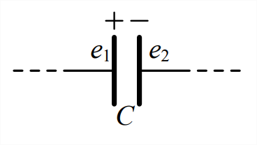
To derive an equation for capacitive potential energy, let us suppose that some quantity of positive charge \(q_{+}\) has already been transferred from the negative plate of an ideal capacitor to the positive plate; the voltage difference between the two plates due to \(q_{+}\) is expressed in terms of the capacitance \(C\), from Equation 5.2.3, as \(e_{1+}-e_{2+}=(1 / C) q_{+}\), in which \(e_{1+}\) is a higher potential than \(e_{2+}\). From Equation \(\ref{eqn:B.23}\), the differential work required to transfer an additional differential quantity of positive charge \(d q_{+}\) from the negative plate to the positive plate is given by
\[d W=d q_{+}\left(e_{1+}-e_{2+}\right)=\frac{1}{C} q_{+} d q_{+}\label{eqn:B.24} \]
We integrate Equation \(\ref{eqn:B.24}\) to find the total work required to fully charge the ideal capacitor from zero to a quantity \(q\), which also is the total electrical potential energy stored in the capacitor:
\[W=E_{E}=\int_{q_{+}=0}^{q_{+}=q} d W=\frac{1}{C} \int_{q_{+}=0}^{q_{+}=q} q_{+} d q_{+}=\frac{1}{2} \frac{1}{C} q^{2}\label{eqn:B.25} \]
Whereas the energy of a capacitor, Equation \(\ref{eqn:B.25}\), is stored in an electrical field, that of an inductor is stored in the magnetic field within the inductor’s coils; this magnetic field exists as a consequence of the electrical current flowing in the wire (Halliday and Resnick, 1960, Chapter 34). Even though it is magnetic field energy, we can still apply Equation \(\ref{eqn:B.23}\) for electrical work to determine an equation for the energy within an inductor (Halliday and Resnick, 1960, Section 36-4). From Equation \(\ref{eqn:B.23}\), the differential work required to move a differential quantity of positive charge through an ideal inductor is
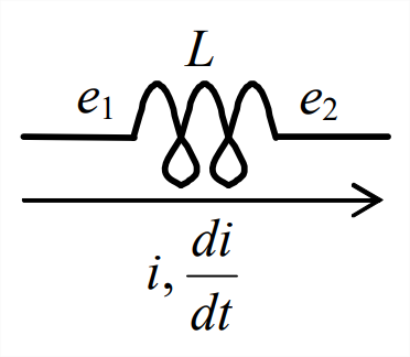
\[d W=d q_{+}\left(e_{1+}-e_{2+}\right)\label{eqn:B.26} \]
in which \(e_{1+}\) is a higher potential than \(e_{2+}\). This is a conservative process, so the electrical work, which might be done by a battery or some other power source, must be stored as magnetic field energy, \(E_{M}\). The self-induced electrical potential difference across the inductor is given by Equation 5.2.9, \(e_{1+}-e_{2+}=L\left(d i_{+} / d t\right)\). Also, current and charge are related by \(i_{+}=d q_{+} / d t\), so that \(d q_{+}=i_{+} d t\). Therefore, we re-write Equation \(\ref{eqn:B.26}\) as
\[d W=d E_{M}=i_{+} d t \times L \frac{d i_{+}}{d t}=L i_{+} d i_{+}\label{eqn:B.27} \]
Finally, we integrate Equation \(\ref{eqn:B.27}\) to find the total magnetic potential energy stored in the ideal inductor for a quantity of current \(i\):
\[W=E_{M}=L \int_{i_{+}=0}^{i_{+}=i} i_{+} d i_{+}=\frac{1}{2} L i^{2}\label{eqn:B.28} \]
Next, we apply Equation \(\ref{eqn:B.23}\) for electrical work once again in order to evaluate power sources and power sinks in electrical circuits (Halliday and Resnick, 1960, Section 31-5). Consider a general component within a circuit, a “black box.” This might be a passive component such as a resistor, a source of power such as a battery or signal generator, or a device such as a motor that converts electrical energy into another form of energy. For this derivation, let us consider the upstream terminal of the black box to be at a higher potential than the downstream terminal: \(e_1 > e_2\). Suppose that a positive differential charge \(dq\) moves through the black box from higher potential to lower potential; Equation \(\ref{eqn:B.23}\) shows that there is a reduction of electrical energy: \(d W=d E_{E}=-d q\left(e_{1}-e_{2}\right)=-i d t\left(e_{1}-e_{2}\right)\). Electrical power also is reduced:
\[P_{E}=\frac{d W}{d t}=-i\left(e_{1}-e_{2}\right)\label{eqn:B.29} \]
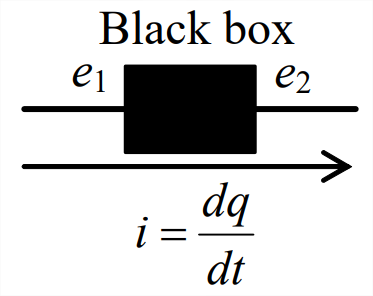
Equation \(\ref{eqn:B.29}\) is an important formula that can be applied usefully for many different black boxes. We shall consider here just two of them. First, suppose that the black box is a resistor with resistance \(R\), for which Equation 5.2.1 gives \(e_{1}-e_{2}=i R\); in this case, the downstream terminal is at lower voltage than the upstream terminal, so Equation \(\ref{eqn:B.29}\) becomes the following famous formula for the electrical power that is dissipated in heating the resistor:
\[P_{R}=-i^{2} R\label{eqn:B.30} \]
Next, suppose that the black box is a source of input voltage \(e_{i}(t)\) (battery or signal generator) for a circuit; in this case, the downstream voltage \(e_{2}=e_{i}(t)\) exceeds the upstream voltage (for positive current \(i\)), so Equation \(\ref{eqn:B.29}\) gives the formula for electrical power introduced into the circuit by the voltage source:
\[P_{e}=i\left[e_{i}(t)-e_{1}\right]\label{eqn:B.31} \]
For most, if not all of the relatively simple circuits considered in this book, the upstream terminal of the voltage source is connected to the ground (zero) potential, so that \(e_{1} \equiv 0\) and the input power is \(P_{e}=i e_{i}(t)\).
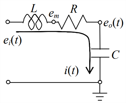
An interesting application of the equations derived in em this section is to the powered \(LRC\) circuit drawn above, from the example in Section 9.2. The total stored electromagnetic energy resides in the electrical field of the ideal capacitor and the magnetic field of the ideal inductor:
\[E_{E M}=E_{E}+E_{M}=\frac{1}{2} \frac{1}{C} q^{2}+\frac{1}{2} L i^{2}\label{eqn:B.32} \]
The signal generator is a source of electrical power, and the resistor is a sink of electrical power, so the total electromagnetic energy varies in time:
\[\frac{d}{d t} E_{E M}=\frac{d}{d t}\left(\frac{1}{2} \frac{1}{C} q^{2}+\frac{1}{2} L i^{2}\right)=P_{R}+P_{e} \Rightarrow L i \frac{d i}{d t}+\frac{1}{C} q \frac{d q}{d t}=-i^{2} R+i e_{i}(t)\label{eqn:B.33} \]
Canceling \(i=\dot{q}\) out of Equation \(\ref{eqn:B.33}\) and re-arranging terms leads to the general ODE for charge \(q(t)\) on the capacitor plates in the \(LRC\) circuit:
\[L \ddot{q}+R \dot{q}+\frac{1}{C} q=e_{i}(t)\label{eqn:B.34} \]
Since \(q=C e_{o}\), Equation \(\ref{eqn:B.34}\) is essentially the same as that derived from Kirchhoff’s voltage law in Section 9.2 for output voltage \(e_{o}(t)\): \(\ddot{e}_{o}+(R / L) \dot{e}_{o}+(1 / L C) e_{o}=(1 / L C) e_{i}(t)\).