
1.1: Signal Classifications and Properties
- Page ID
- 22837

Introduction
This module will begin our study of signals and systems by laying out some of the fundamentals of signal classification. It is essentially an introduction to the important definitions and properties that are fundamental to the discussion of signals and systems, with a brief discussion of each.
Classifications of Signals
Continuous-Time vs. Discrete-Time
As the names suggest, this classification is determined by whether or not the time axis is discrete (countable) or continuous (Figure \(\PageIndex{1}\)). A continuous-time signal will contain a value for all real numbers along the time axis. In contrast to this, a discrete-time signal, often created by sampling a continuous signal, will only have values at equally spaced intervals along the time axis.
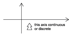
Figure \(\PageIndex{1}\)
Analog vs. Digital
The difference between analog and digital is similar to the difference between continuous-time and discrete-time. However, in this case the difference involves the values of the function. Analog corresponds to a continuous set of possible function values, while digital corresponds to a discrete set of possible function values. An common example of a digital signal is a binary sequence, where the values of the function can only be one or zero.
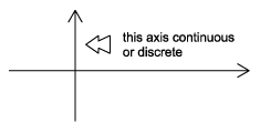
Figure \(\PageIndex{2}\)
Periodic vs. Aperiodic
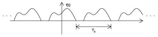
Periodic signals repeat with some period \(T\), while aperiodic, or nonperiodic, signals do not (Figure \(\PageIndex{3}\)). We can define a periodic function through the following mathematical expression, where \(t\) can be any number and \(T\) is a positive constant:
\[f(t)=f(t+T) \label{1.1} \]
fundamental period of our function, \(f(t)\), is the smallest value of \(T\) that the still allows Equation \ref{1.1} to be true.
 (b)
(b)
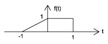
Finite vs. Infinite Length
Another way of classifying a signal is in terms of its length along its time axis. Is the signal defined for all possible values of time, or for only certain values of time? Mathematically speaking, \(f(t)\) is a finite-length signal if it is defined only over a finite interval
\[ t_{1}<t<t_{2} \nonumber \]
where \(t_1 < t_2\). Similarly, an infinite-length signal, \(f(t)\), is defined for all values:
\[ -\infty<t<\infty \nonumber \]
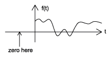
Causal vs. Anticausal vs. Noncausal
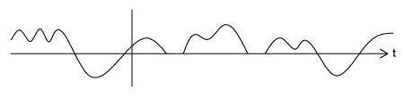
Causal signals are signals that are zero for all negative time, while anticausal are signals that are zero for all positive time. Noncausal signals are signals that have nonzero values in both positive and negative time (Figure \(\PageIndex{4}\)).
 (a)
(a)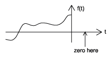 (b)
(b)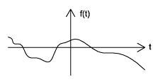 (c)
(c)
Even vs. Odd
An even signal is any signal \(f\) such that \(f(t) = f(-t)\). Even signals can be easily spotted as they are symmetric around the vertical axis. An odd signal, on the other hand, is a signal \(f\) such that \(f(t)=−f(−t)\) (Figure \(\PageIndex{5}\)).
 (a)
(a)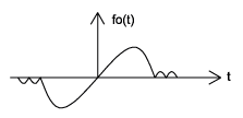 (b)
(b)
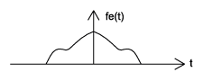
Using the definitions of even and odd signals, we can show that any signal can be written as a combination of an even and odd signal. That is, every signal has an odd-even decomposition. To demonstrate this, we have to look no further than a single equation.
\[ f(t)=\frac{1}{2}(f(t)+f(-t))+\frac{1}{2}(f(t)-f(-t)) \label{1.2} \]
By multiplying and adding this expression out, it can be shown to be true. Also, it can be shown that \(f(t)+f(−t)\) fulfills the requirement of an even function, while \(f(t)−f(−t)\) fulfills the requirement of an odd function (Figure \(\PageIndex{6}\)).
 (a)
(a)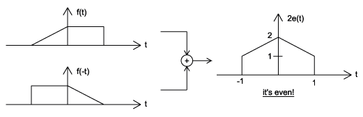 (b)
(b)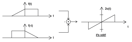 (c)
(c)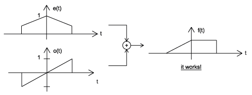 (d)
(d)
Deterministic vs. Random
A deterministic signal is a signal in which each value of the signal is fixed, being determined by a mathematical expression, rule, or table. On the other hand, the values of a random signal are not strictly defined, but are subject to some amount of variability.
 (b)
(b)
Consider the signal defined for all real \(t\) described by
\[f(t)=\left\{\begin{array}{cc}
\sin (2 \pi t) / t & t \geq 1 \\
0 & t<1
\end{array}\right. \nonumber \]
This signal is continuous time, analog, aperiodic, infinite length, causal, neither even nor odd, and, by definition, deterministic.
Signal Classifications Summary
This module describes just some of the many ways in which signals can be classified. They can be continuous time or discrete time, analog or digital, periodic or aperiodic, finite or infinite, and deterministic or random. We can also divide them based on their causality and symmetry properties.