3.7: Linear Constant Coefficient Differential Equations

Introduction: Ordinary Differential Equations

In our study of signals and systems, it will often be useful to describe systems using equations involving the rate of change in some quantity. Such equations are called differential equations. For instance, you may remember from a past physics course that an object experiences simple harmonic motion when it has an acceleration that is proportional to the magnitude of its displacement and opposite in direction. Thus, this system is described as the differential equation shown in Equation \ref{3.58}.

\[\frac{d^{2} x}{d t^{2}}=-c x \label{3.58} \]

Because the differential equation in Equation \ref{3.58} has only one independent variable and only has derivatives with respect to that variable, it is called an ordinary differential equation. There are more complicated differential equations, such as the Schrödinger equation, which involve derivatives with respect to multiple independent variables. These are called partial differential equations, but they are not within the scope of this module.

Given a sufficiently descriptive set of initial conditions or boundary conditions, if there is a solution to the differential equation, that solution is unique and describes the behavior of the system. Of course, the results are only accurate to the degree that the model mirrors reality.

Linear Constant Coefficient Ordinary Differential Equations

An important subclass of ordinary differential equations is the set of linear constant coefficient ordinary differential equations. These equations are of the form

\[A x(t)=f(t) \label{3.59} \]

where \(A\) is a differential operator of the form given in Equation \ref{3.60}.

\[A=a_{n} \frac{d^{n}}{d t^{n}}+a_{n-1} \frac{d^{n-1}}{d t^{n-1}}+\ldots+a_{1} \frac{d}{d t}+a_{0} \label{3.60} \]

Note that operators of this type satisfy the linearity conditions, and \(a_1,...,a_n\) are real constants. Furthermore, Equation \ref{3.59} with these operators has derivatives with respect to only one variable, making it an ordinary differential equation.

A similar concept for a discrete time setting, difference equations, is discussed in the chapter on time domain analysis of discrete time systems. There are many parallels between the discussion of linear constant coefficient ordinary differential equations and linear constant coefficient difference equations.

Applications of Differential Equations

Consider the decay model in which a quantity of an unstable isotope decreases at a rate proportional to the quantity of unstable isotope remaining. Thus, the decay of the isotope is modeled by the first order linear constant coefficient differential equation

\[\frac{d x}{d t}+r x=0 \nonumber \]

where \(r\) is some real rate.

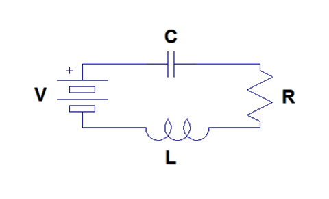
Now consider the series RLC circuit shown in Figure \(\PageIndex{1}\). This system can be modeled using differential equations. We can use the voltage equations for each circuit element and Kirchoff's voltage law to write a second order linear constant coefficient differential equation describing the charge on the capacitor.

The voltage across the battery is simply \(V\). The voltage across the capacitor is \(\frac{1}{C}q\). The voltage across the resistor is \(R\frac{dq}{dt}\). Finally, the voltage across the inductor is \(L\frac{d^2q}{dt^2}\). Therefore, by Kirchoff's voltage law, it follows that

\[L \frac{d^{2} q}{d t^{2}}+R \frac{d q}{d t}+\frac{1}{C} q=V. \nonumber \]

Figure \(\PageIndex{1}\): A series RLC circuit.

The section Solving Linear Constant Coefficient Differential Equations will describe in depth how solutions to differential equations like those in the examples may be obtained.

Linear Constant Coefficient Ordinary Differential Equations Summary

Differential equations are an important mathematical tool for modeling continuous time systems. An important subclass of these is the class of linear constant coefficient ordinary differential equations. Linear constant coefficient ordinary differential equations are often particularly easy to solve as will be described in the module on solutions to linear constant coefficient ordinary differential equations and are useful in describing a wide range of situations that arise in electrical engineering and in other fields.