3.8: Solving Linear Constant Coefficient Differential Equations

Introduction

The approach to solving linear constant coefficient ordinary differential equations is to find the general form of all possible solutions to the equation and then apply a number of conditions to find the appropriate solution. The two main types of problems are initial value problems, which involve constraints on the solution and its derivatives at a single point, and boundary value problems, which involve constraints on the solution or its derivatives at several points.

The number of initial conditions needed for an \(N\)th order differential equation, which is the order of the highest order derivative, is \(N\), and a unique solution is always guaranteed if these are supplied. Boundary value problems can be slightly more complicated and will not necessarily have a unique solution or even a solution at all for a given set of conditions. Thus, this module will focus exclusively on initial value problems.

Solving Linear Constant Coefficient Ordinary Differential Equations

Consider some linear constant coefficient ordinary differential equation given by \(Ax(t)=f(t)\), where \(A\) is a differential operator of the form

\[A=a_{n} \frac{d^{n}}{d t^{n}}+a_{n-1} \frac{d^{n-1}}{d t^{n-1}}+\ldots+a_{1} \frac{d}{d t}+a_{0} \nonumber \]

Let \(x_h(t)\) and \(x_p(t)\) be two functions such that \(Ax_h(t)=0\) and \(Ax_p(t)=f(t)\). By the linearity of \(A\), note that \(A(x_h(t)+x_p(t))=0+f(t)=f(t)\). Thus, the form of the general solution \(x_g(t)\) to any linear constant coefficient ordinary differential equation is the sum of a homogeneous solution \(x_h(t)\) to the equation \(Ax=0\) and a particular solution \(x_p(t)\) that is specific to the forcing function \(f(t)\).

We wish to determine the forms of the homogeneous and nonhomogeneous solutions in full generality in order to avoid incorrectly restricting the form of the solution before applying any conditions. Otherwise, a valid set of initial or boundary conditions might appear to have no corresponding solution trajectory. The following discussion shows how to accomplish this for linear constant coefficient ordinary differential equations.

Finding the Homogeneous Solution

In order to find the homogeneous solution to \(Ax(t)=f(t)\), consider the differential equation \(Ax(t)=0\). We know that the solutions have the form \(ce^{\lambda t}\) for some complex constants \(c\), \(\lambda\). Since \(Ace^{\lambda t} = 0\) for a solution, it follows that

\[\left(a_{n} \frac{d^{n}}{d t^{n}}+a_{n-1} \frac{d^{n-1}}{d t^{n-1}}+\ldots+a_{1} \frac{d}{d t}+a_{0}\right) e^{\lambda t}=0, \nonumber \]

so it also follows that

\[a_{n} \lambda^{n}+a_{n-1} \lambda^{n-1} \ldots+a_{1} \lambda+a_{0}=0. \nonumber \]

Therefore, the parameters of the solution exponents are the roots of the above polynomial, called the characteristic polynomial.

For equations of order two or more, there will be several roots. If all of the roots are distinct, then the the general form of the homogeneous solution is simply

\[x_{h}(t)=c_{1} e^{\lambda_{1} t}+\ldots+c_{n} e^{\lambda_{n} t}. \nonumber \]

If a root has multiplicity that is greater than one, the repeated solutions must be multiplied by each powers of \(t\) from 0 to one less than the root multiplicity (in order to ensure linearly independent solutions). For instance, if \(\lambda_1\) had multiplicity 2 and \(\lambda_2\) had multiplicity 3, the homogeneous solution would be

\[x_{h}(t)=c_{1} e^{\lambda_{1} t}+c_{2} t e^{\lambda_{1} t}+c_{3} e^{\lambda_{2} t}+c_{4} t e^{\lambda_{2} t}+c_{5} t^{2} e^{\lambda_{2} t} \nonumber \]

Example \(\PageIndex{1}\)

Consider the decay model in which a quantity of an unstable isotope decreases at a rate proportional to the quanity of unstable isotope remaining. Thus, the decay of the isotope is modeled by the first order linear constant coefficient differential equation

\[\frac{d x}{d t}+r x=0 \nonumber \]

where \(r\) is some real rate. This differential equation could easily be solved through straightforward integration. However, the methods described above will be used instead. Note that the forcing function is zero, so only a homogenous solution is needed. It is easy to see that the characteristic polynomial is \(\lambda+r=0\), so there is one root \(\lambda_1=r\). Thus the solution is of the form

\[x(t)=c_{1} e^{r t} \nonumber \]

Given a rate and an initial condition, this can be applied to a specific situation. For instance, we know that carbon-14 decays at a rate of approximately \(r=1.21\times 10^{−4}\) year\(^{−1}\), and if we normalize the natural concentration of carbon-14 to \(x(0)=1\) the solution becomes \(x(t)=e^{−1.21\times 10^{−4}t}\). Knowledge of this curve would be useful for radioisotope based dating.

Finding the Particular Solution

Finding the particular solution is slightly more complicated task than finding the homogeneous solution. A formal method, called variation of parameters accomplishes this, and there are also several heuristics that can be used. It can also be found through convolution of the input with the unit impulse response, once the unit impulse response is known. Finding the particular solution to a differential equation is discussed further in the chapter concerning the Laplace transform, which greatly simplifies the procedure for solving linear constant coefficient ordinary differential equations using frequency domain tools.

Example \(\PageIndex{2}\)

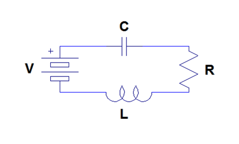
Consider the series RLC circuit shown in Figure \(\PageIndex{1}\). This system can be modeled using differential equations. We can use the voltage equations for each circuit element and Kirchoff's voltage law to write a second order linear constant coefficient differential equation describing the charge on the capacitor.

The voltage across the battery is simply \(V\). The voltage across the capacitor is \(\frac{1}{C}q\). The voltage across the resistor is \(R \frac{dq}{dt}\). Finally, the voltage across the inductor is \(L\frac{d^2q}{dt^2}\). Therefore, by Kirchoff's voltage law, it follows that

\[L \frac{d^{2} q}{d t^{2}}+R \frac{d q}{d t}+\frac{1}{C} q=V \nonumber \]

Figure \(\PageIndex{1}\): A series RLC circuit.

First, the homogeneous solution is found. It is easy to see that the characteristic polynomial is \(L \lambda^{2}+R \lambda+\frac{1}{C}=0\). Therefore, the two roots are \(\lambda_{1}=\frac{-R-\sqrt{R^{2}-\frac{4 L}{C}}}{2 L}\) and \(\lambda_{2}=\frac{-R+\sqrt{R^{2}-\frac{4 L}{C}}}{2 L}\). Often, these are stated in terms of the attenuation factor \(\alpha=\frac{R}{2} \sqrt{\frac{C}{L}}\) and the resonant frequency \(\omega_{0}=\frac{1}{\sqrt{L C}}\). Thus, \(\lambda_{1}=-\alpha-\sqrt{\alpha^{2}-\omega_{0}^{2}}\) and \(\lambda_{2}=-\alpha+\sqrt{\alpha^{2}-\omega_{0}^{2}}\).

Thus, the homogeneous equation is of the form

\[ x_{h}(t)=c_{1} e^{-\alpha-\sqrt{\alpha^{2}-\omega_{0}^{2}}}+c_{2} e^{-\alpha+\sqrt{\alpha^{2}-\omega_{0}^{2}}}. \nonumber \]

It turns out that the response to the constant voltage source forcing function is a constant, so

\[x_{p}(t)=V C. \nonumber \]

Hence, the general solution is

\[x(t)=V C+c_{1} e^{-\alpha-\sqrt{\alpha^{2}-\omega_{0}^{2}} t}+c_{2} e^{-\alpha+\sqrt{\alpha^{2}-\omega_{0}^{2}} t} \nonumber \]

where \(c_1\) and \(c_2\) depend on the initial conditions. The system demonstrates a rich array of behaviors based on the relative values of \(\alpha\) and \(\omega_0\), which the reader is encouraged to explore.

Solving Differential Equations Summary

Linear constant coefficient ordinary differential equations are useful for modeling a wide variety of continuous time systems. The approach to solving them is to find the general form of all possible solutions to the equation and then apply a number of conditions to find the appropriate solution. This is done by finding the homogeneous solution to the differential equation that does not depend on the forcing function input and a particular solution to the differential equation that does depend on the forcing function input.