
4.3: Discrete Time Convolution
- Page ID
- 22860

Introduction
Convolution, one of the most important concepts in electrical engineering, can be used to determine the output a system produces for a given input signal. It can be shown that a linear time invariant system is completely characterized by its impulse response. The sifting property of the discrete time impulse function tells us that the input signal to a system can be represented as a sum of scaled and shifted unit impulses. Thus, by linearity, it would seem reasonable to compute of the output signal as the sum of scaled and shifted unit impulse responses. That is exactly what the operation of convolution accomplishes. Hence, convolution can be used to determine a linear time invariant system's output from knowledge of the input and the impulse response.
Convolution and Circular Convolution
Convolution
Operation Definition
Discrete time convolution is an operation on two discrete time signals defined by the integral
\[(f * g)[n]=\sum_{k=-\infty}^{\infty} f[k] g[n-k] \nonumber \]
for all signals \(f\), \(g\) defined on \(\mathbb{Z}\). It is important to note that the operation of convolution is commutative, meaning that
\[f * g=g * f \nonumber \]
for all signals \(f\), \(g\) defined on \(\mathbb{Z}\). Thus, the convolution operation could have been just as easily stated using the equivalent definition
\[(f * g)[n]=\sum_{k=-\infty}^{\infty} f[n-k] g[k] \nonumber \]
for all signals \(f\), \(g\) defined on \(\mathbb{Z}\). Convolution has several other important properties not listed here but explained and derived in a later module.
Definition Motivation
The above operation definition has been chosen to be particularly useful in the study of linear time invariant systems. In order to see this, consider a linear time invariant system \(H\) with unit impulse response \(h\). Given a system input signal \(x\) we would like to compute the system output signal \(H(x)\). First, we note that the input can be expressed as the convolution
\[x[n]=\sum_{k=-\infty}^{\infty} x[k] \delta[n-k] \nonumber \]
by the sifting property of the unit impulse function. By linearity
\[ H(x[n])=\sum_{k=-\infty}^{\infty} x[k] H(\delta[n-k]). \nonumber \]
Since \(H(\delta[n-k])\) is the shifted unit impulse response \(h[n−k]\), this gives the result
\[ H(x[n])=\sum_{k=-\infty}^{\infty} x[k] h[n-k]=(x * h)[n]. \nonumber \]
Hence, convolution has been defined such that the output of a linear time invariant system is given by the convolution of the system input with the system unit impulse response.
Graphical Intuition
It is often helpful to be able to visualize the computation of a convolution in terms of graphical processes. Consider the convolution of two functions \(f\), \(g\) given by
\[(f * g)[n]=\sum_{k=-\infty}^{\infty} f[k] g[n-k]=\sum_{k=-\infty}^{\infty} f[n-k] g[k]. \nonumber \]
The first step in graphically understanding the operation of convolution is to plot each of the functions. Next, one of the functions must be selected, and its plot reflected across the \(k=0\) axis. For each real \(n\), that same function must be shifted left by \(n\). The point-wise product of the two resulting plots is then computed, and then all of the values are summed.
Example \(\PageIndex{1}\)
Recall that the impulse response for a discrete time echoing feedback system with gain \(a\) is
\[h[n]=a^{n} u[n], \nonumber \]
and consider the response to an input signal that is another exponential
\[x[n]=b^{n} u[n] . \nonumber \]
We know that the output for this input is given by the convolution of the impulse response with the input signal
\[y[n]=x[n] * h[n]. \nonumber \]
We would like to compute this operation by beginning in a way that minimizes the algebraic complexity of the expression. However, in this case, each possible choice is equally simple. Thus, we would like to compute
\[ y[n]=\sum_{k=-\infty}^{\infty} a^{k} u[k] b^{n-k} u[n-k]. \nonumber \]
The step functions can be used to further simplify this sum. Therefore,
\[y[n]=0 \nonumber \]
for \(n<0\) and
\[y[n]=\sum_{k=0}^{n}[a b]^{k} \nonumber \]
for \(n \geq 0\). Hence, provided \(a b \neq 1\), we have that
\[y[n]=\left\{\begin{array}{cc}
0 & n<0 \\
\frac{1-(a b)^{n+1}}{1-(a b)} & n \geq 0
\end{array}\right. \nonumber \]
Circular Convolution
Discrete time circular convolution is an operation on two finite length or periodic discrete time signals defined by the sum
\[(f \circledast g)[n]=\sum_{k=0}^{N-1} \hat{f}[k] \hat{g}[n-k] \nonumber \]
for all signals \(f\), \(g\) defined on \(\mathbb{Z}[0, N-1]\) where \(\hat{f}\), \(\hat{g}\) are periodic extensions of \(f\) and \(g\). It is important to note that the operation of circular convolution is commutative, meaning that
\[f \circledast g = g \circledast f \nonumber \]
for all signals \(f\), \(g\) defined on \(\mathbb{Z}[0, N-1]\). Thus, the circular convolution operation could have been just as easily stated using the equivalent definition
\[(f \circledast g)[n]=\sum_{k=0}^{N-1} \hat{f}[n-k] \hat{g}[k] \nonumber \]
for all signals \(f\), \(g\) defined on \(\mathbb{Z}[0, N-1]\) where \(\hat{f}\), \(\hat{g}\) are periodic extensions of \(f\) and \(g\). Circular convolution has several other important properties not listed here but explained and derived in a later module.
Alternatively, discrete time circular convolution can be expressed as the sum of two summations given by
\[(f \circledast g)[n]=\sum_{k=0}^{n} f[k] g[n-k]+\sum_{k=n+1}^{N-1} f[k] g[n-k+N] \nonumber \]
for all signals \(f\), \(g\) defined on \(\mathbb{Z}[0, N-1]\).
Meaningful examples of computing discrete time circular convolutions in the time domain would involve complicated algebraic manipulations dealing with the wrap around behavior, which would ultimately be more confusing than helpful. Thus, none will be provided in this section. Of course, example computations in the time domain are easy to program and demonstrate. However, discrete time circular convolutions are more easily computed using frequency domain tools as will be shown in the discrete time Fourier series section.
Definition Motivation
The above operation definition has been chosen to be particularly useful in the study of linear time invariant systems. In order to see this, consider a linear time invariant system \(H\) with unit impulse response \(h\). Given a periodic system input signal \(x\) we would like to compute the system output signal \(H(x)\). First, we note that the input can be expressed as the circular convolution
\[x[n]=\sum_{k=0}^{N-1} \widehat{x}[k] \hat{\delta}[n-k] \nonumber \]
by the sifting property of the unit impulse function. By linearity,
\[H(x[n])=\sum_{k=0}^{N-1} \widehat{x}[k] H(\hat{\delta}[n-k]). \nonumber \]
Since \(H(\delta[n-k])\) is the shifted unit impulse response \(h[n−k]\), this gives the result
\[ H(x[n])=\sum_{k=0}^{N-1} \hat{x}[k] \hat{h}[n-k]=(x \circledast h)[n]. \nonumber \]
Hence, circular convolution has been defined such that the output of a linear time invariant system is given by the convolution of the system input with the system unit impulse response.
Graphical Intuition
It is often helpful to be able to visualize the computation of a circular convolution in terms of graphical processes. Consider the circular convolution of two finite length functions \(f\), \(g\) given by
\[(f \circledast g)[n]=\sum_{k=0}^{N-1} \hat{f}[k] \hat{g}[n-k]=\sum_{k=0}^{N-1} \hat{f}[n-k] \hat{g}[k] \nonumber \]
The first step in graphically understanding the operation of convolution is to plot each of the periodic extensions of the functions. Next, one of the functions must be selected, and its plot reflected across the \(k=0\) axis. For each \(n \in \mathbb{Z}[0, N-1]\), that same function must be shifted left by \(n\). The point-wise product of the two resulting plots is then computed, and finally all of these values are summed.
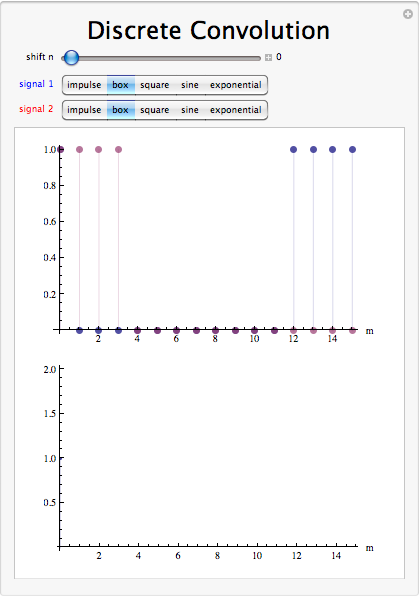
Interactive Element
Convolution Summary
Convolution, one of the most important concepts in electrical engineering, can be used to determine the output signal of a linear time invariant system for a given input signal with knowledge of the system's unit impulse response. The operation of discrete time convolution is defined such that it performs this function for infinite length discrete time signals and systems. The operation of discrete time circular convolution is defined such that it performs this function for finite length and periodic discrete time signals. In each case, the output of the system is the convolution or circular convolution of the input signal with the unit impulse response.