
6.7: Gibbs Phenomena
- Page ID
- 23141

Introduction
The Fourier Series is the representation of continuous-time, periodic signals in terms of complex exponentials. The Dirichlet conditions suggest that discontinuous signals may have a Fourier Series representation so long as there are a finite number of discontinuities. This seems counter-intuitive, however, as complex exponentials (Section 1.8) are continuous functions. It does not seem possible to exactly reconstruct a discontinuous function from a set of continuous ones. In fact, it is not. However, it can be if we relax the condition of 'exactly' and replace it with the idea of 'almost everywhere'. This is to say that the reconstruction is exactly the same as the original signal except at a finite number of points. These points, not necessarily surprisingly, occur at the points of discontinuities.
History
In the late 1800s, many machines were built to calculate Fourier coefficients and re-synthesize:
\[f_{N}^{\prime}(t)=\sum_{n=-N}^{N} c_{n} e^{j \omega_{0} n t} \nonumber \]
Albert Michelson (an extraordinary experimental physicist) built a machine in 1898 that could compute \(c_n\) up to \(n=\pm(79)\), and he re-synthesized
\[f_{79}^{\prime}(t)=\sum_{n=-79}^{79} c_{n} e^{j \omega_{0} n t} \nonumber \]
The machine performed very well on all tests except those involving discontinuous functions. When a square wave, like that shown in Figure \(\PageIndex{1}\), was inputted into the machine, "wiggles" around the discontinuities appeared, and even as the number of Fourier coefficients approached infinity, the wiggles never disappeared - these can be seen in the last plot in Figure \(\PageIndex{1}\). J. Willard Gibbs first explained this phenomenon in 1899, and therefore these discontinuous points are referred to as Gibbs Phenomenon.
Explanation
We begin this discussion by taking a signal with a finite number of discontinuities (like a square pulse) and finding its Fourier Series representation. We then attempt to reconstruct it from these Fourier coefficients. What we find is that the more coefficients we use, the more the signal begins to resemble the original. However, around the discontinuities, we observe rippling that does not seem to subside. As we consider even more coefficients, we notice that the ripples narrow, but do not shorten. As we approach an infinite number of coefficients, this rippling still does not go away. This is when we apply the idea of almost everywhere. While these ripples remain (never dropping below 9% of the pulse height), the area inside them tends to zero, meaning that the energy of this ripple goes to zero. This means that their width is approaching zero and we can assert that the reconstruction is exactly the original except at the points of discontinuity. Since the Dirichlet conditions assert that there may only be a finite number of discontinuities, we can conclude that the principle of almost everywhere is met. This phenomenon is a specific case of nonuniform convergence.
Below we will use the square wave, along with its Fourier Series representation, and show several figures that reveal this phenomenon more mathematically.
Square Wave
The Fourier series representation of a square signal below says that the left and right sides are "equal." In order to understand Gibbs Phenomenon we will need to redefine the way we look at equality.
\[s(t)=a_{0}+\sum_{k=1}^{\infty} a_{k} \cos \left(\frac{2 \pi k t}{T}\right)+\sum_{k=1}^{\infty} b_{k} \sin \left(\frac{2 \pi k t}{T}\right) \nonumber \]
Figure \(\PageIndex{1}\) shows several Fourier series approximations of the square wave using a varied number of terms, denoted by KK:
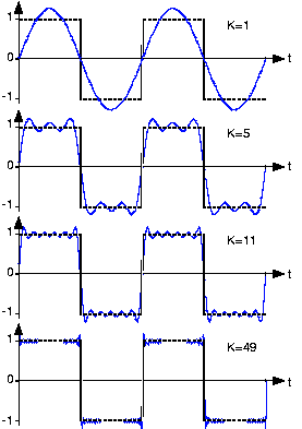
When comparing the square wave to its Fourier series representation in Figure \(\PageIndex{1}\), it is not clear that the two are equal. The fact that the square wave's Fourier series requires more terms for a given representation accuracy is not important. However, close inspection of Figure \(\PageIndex{1}\) does reveal a potential issue: Does the Fourier series really equal the square wave at all values of tt? In particular, at each step-change in the square wave, the Fourier series exhibits a peak followed by rapid oscillations. As more terms are added to the series, the oscillations seem to become more rapid and smaller, but the peaks are not decreasing. Consider this mathematical question intuitively: Can a discontinuous function, like the square wave, be expressed as a sum, even an infinite one, of continuous ones? One should at least be suspicious, and in fact, it can't be thus expressed. This issue brought Fourier much criticism from the French Academy of Science (Laplace, Legendre, and Lagrange comprised the review committee) for several years after its presentation on 1807. It was not resolved for also a century, and its resolution is interesting and important to understand from a practical viewpoint.
The extraneous peaks in the square wave's Fourier series never disappear; they are termed Gibb's phenomenon after the American physicist Josiah Willard Gibbs. They occur whenever the signal is discontinuous, and will always be present whenever the signal has jumps.
Redefine Equality
Let's return to the question of equality; how can the equal sign in the definition of the Fourier series (Section 4.3) be justified? The partial answer is that pointwise--each and every value of \(t\)--equality is not guaranteed. What mathematicians later in the nineteenth century showed was that the rms error of the Fourier series was always zero.
\[\lim_{K \rightarrow \infty} \operatorname{rms}\left(\varepsilon_{K}\right)=0 \nonumber \]
What this means is that the difference between an actual signal and its Fourier series representation may not be zero, but the square of this quantity has zero integral! It is through the eyes of the rms value that we define equality: Two signals \(s_1(t)\), \(s_2(t)\) are said to be equal in the mean square if rms \((s_1−s_2)=0\). These signals are said to be equal pointwise if \(s_1(t)=s_2(t)\) for all values of \(t\). For Fourier series, Gibb's phenomenon peaks have finite height and zero width: The error differs from zero only at isolated points--whenever the periodic signal contains discontinuities--and equals about 9% of the size of the discontinuity. The value of a function at a finite set of points does not affect its integral. This effect underlies the reason why defining the value of a discontinuous function at its discontinuity is meaningless. Whatever you pick for a value has no practical relevance for either the signal's spectrum or for how a system responds to the signal. The Fourier series value "at" the discontinuity is the average of the values on either side of the jump.
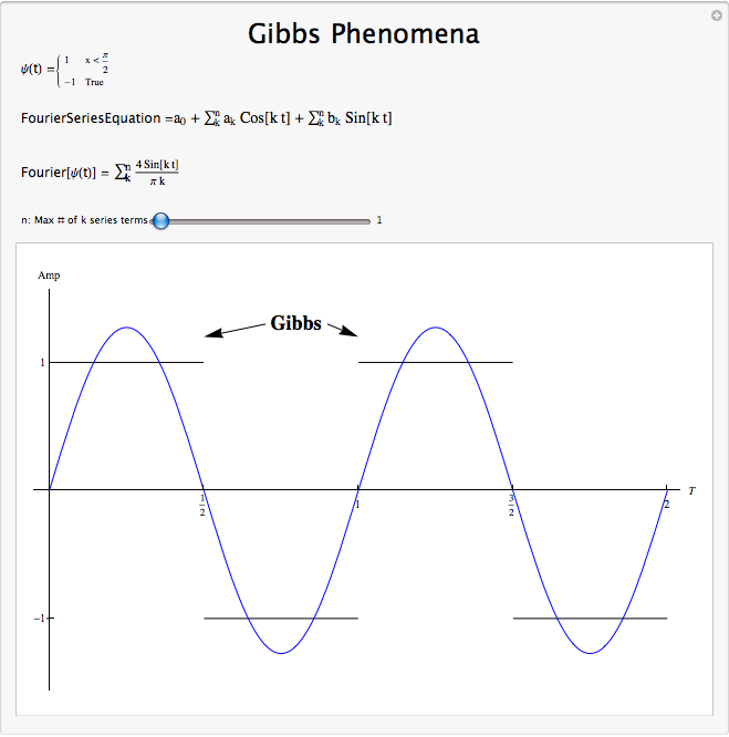
Visualizing Gibb's Phenomena
The following VI demonstrates the occurrence of Gibb's Phenomena. Note how the wiggles near the square pulse to the left remain even if you drastically increase the order of the approximation, even though they do become narrower. Also notice how the approximation of the smooth region in the middle is much better than that of the discontinuous region, especially at lower orders.
Conclusion
We can approximate a function by re-synthesizing using only some of the Fourier coefficients (truncating the F.S.)
\[f_{N}^{\prime}(t)=\sum_{n n \leq|N|} c_{n} e^{j \omega_{0} n t} \nonumber \]
This approximation works well where \(f(t)\) is continuous, but not so well where \(f(t)\) is discontinuous. In the regions of discontinuity, we will always find Gibb's Phenomena, which never decrease below 9% of the height of the discontinuity, but become narrower and narrower as we add more terms.