9.2: Discrete Time Fourier Transform (DTFT)

Introduction

In this module, we will derive an expansion for arbitrary discrete-time functions, and in doing so, derive the Discrete Time Fourier Transform (DTFT).

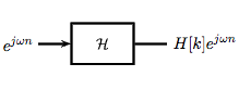
Since complex exponentials (Section 1.8) are eigenfunctions of linear time-invariant (LTI) systems (Section 14.5), calculating the output of an LTI system \(\mathcal{H}\) given \(e^{j \omega n}\) as an input amounts to simple multiplication, where \(\omega_{0}=\frac{2 \pi k}{N}\), and where \(H[k] \in \mathrm{C}\) is the eigenvalue corresponding to \(k\). As shown in the figure, a simple exponential input would yield the output

\[y[n]=H[k] e^{j \omega n} \nonumber \]

Figure \(\PageIndex{1}\): Simple LTI system.

Using this and the fact that \(\mathcal{H}\) is linear, calculating \(y[n]\) for combinations of complex exponentials is also straightforward.

\[\begin{array}{c}
c_{1} e^{j \omega_{1} n}+c_{2} e^{j \omega_{2} n} \rightarrow c_{1} H\left[k_{1}\right] e^{j \omega_{1} n}+c_{2} H\left[k_{2}\right] e^{j \omega_{1} n} \\
\sum_{l} c_{l} e^{j \omega_{l}n} \rightarrow \sum_{l} c_{l} H\left[k_{l}\right] e^{j \omega_{l} n}
\end{array} \nonumber \]

The action of \(H\) on an input such as those in the two equations above is easy to explain. \(\mathbf{\mathcal{H}}\) independently scales each exponential component \(e^{j \omega_{l} n}\) by a different complex number \(H\left[k_{l}\right] \in \mathbb{C}\). As such, if we can write a function \(y[n]\) as a combination of complex exponentials it allows us to easily calculate the output of a system.

Now, we will look to use the power of complex exponentials to see how we may represent arbitrary signals in terms of a set of simpler functions by superposition of a number of complex exponentials. Below we will present the Discrete-Time Fourier Transform (DTFT). Because the DTFT deals with nonperiodic signals, we must find a way to include all real frequencies in the general equations. For the DTFT we simply utilize summation over all real numbers rather than summation over integers in order to express the aperiodic signals.

DTFT synthesis

It can be demonstrated that an arbitrary Discrete Time-periodic function \(f[n]\) can be written as a linear combination of harmonic complex sinusoids

\[f[n]=\sum_{k=0}^{N-1} c_{k} e^{j \omega_{0} k n} \label{9.3} \]

where \(\omega_{0}=\frac{2 \pi}{N}\) is the fundamental frequency. For almost all \(f[n]\) of practical interest, there exists \(c_n\) to make Equation \ref{9.3} true. If \(f[n]\) is finite energy ( \(f[n] \in L^{2}[0, N]\) ), then the equality in Equation \ref{9.3} holds in the sense of energy convergence; with discrete-time signals, there are no concerns for divergence as there are with continuous-time signals.

The \(c_n\) - called the Fourier coefficients - tell us "how much" of the sinusoid \(e^{j \omega_{0} kn}\) is in \(f[n]\). The formula shows \(f[n]\) as a sum of complex exponentials, each of which is easily processed by an LTI system (since it is an eigenfunction of every LTI system). Mathematically, it tells us that the set of complex exponentials \(\left\{e^{j \omega_{0} k n}, k \in \mathbb{Z}\right\}\) form a basis for the space of N-periodic discrete time functions.

Equations

Now, in order to take this useful tool and apply it to arbitrary non-periodic signals, we will have to delve deeper into the use of the superposition principle. Let \(s_T(t)\) be a periodic signal having period \(T\). We want to consider what happens to this signal's spectrum as the period goes to infinity. We denote the spectrum for any assumed value of the period by \(c_n(T)\). We calculate the spectrum according to the Fourier formula for a periodic signal, known as the Fourier Series (for more on this derivation, see the section on Fourier Series.)

\[c_{n}=\frac{1}{T} \int_{0}^{T} s(t) \exp \left(-j \omega_{0} t\right) d t \nonumber \]

where \(\omega_0 = \frac{2 \pi}{T}\) and where we have used a symmetric placement of the integration interval about the origin for subsequent derivational convenience. We vary the frequency index \(n\) proportionally as we increase the period. Define

\[S_{T}(f) \equiv T c_{n}=\frac{1}{T} \int_{0}^{T} S_{T}(f) \exp \left(j \omega_{0} t\right) d t \nonumber \]

making the corresponding Fourier Series

\[s_{T}(t)=\sum_{-\infty}^{\infty} f(t) \exp \left(j \omega_{0} t\right) \frac{1}{T} \nonumber \]

As the period increases, the spectral lines become closer together, becoming a continuum. Therefore,

\[\lim _{T \rightarrow \infty} s_{T}(t) \equiv s(t)=\int_{-\infty}^{\infty} S(f) \exp \left(j \omega_{0} t\right) d f \nonumber \]

with

\[S(f)=\int_{-\infty}^{\infty} s(t) \exp \left(-j \omega_{0} t\right) d t \nonumber \]

Discrete-Time Fourier Transform

\[\mathcal{F}(\omega)=\sum_{n=-\infty}^{\infty} f[n] e^{-(j \omega n)} \nonumber \]

Inverse DTFT

\[f[n]=\frac{1}{2 \pi} \int_{-\pi}^{\pi} \mathcal{F}(\omega) e^{j \omega n} d \omega \nonumber \]

Warning

It is not uncommon to see the above formula written slightly different. One of the most common differences is the way that the exponential is written. The above equations use the radial frequency variable \(\omega\) in the exponential, where \(\omega = 2 \pi f\), but it is also common to include the more explicit expression, \(j 2 \pi f t\), in the exponential. Sometimes DTFT notation is expressed as \(F(e^{j \omega})\), to make it clear that it is not a CTFT (which is denoted as \(F(\Omega)\). Click here for an overview of the notation used in Connexion's DSP modules.

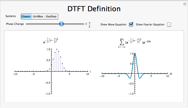
DTFT Definition demonstration

Figure \(\PageIndex{2}\): Click on the above thumbnail image (when online) to download an interactive Mathematica Player demonstrating Discrete Time Fourier Transform. To Download, right-click and save target as .cdf.

DTFT Summary

Because complex exponentials are eigenfunctions of LTI systems, it is often useful to represent signals using a set of complex exponentials as a basis. The discrete time Fourier transform synthesis formula expresses a discrete time, aperiodic function as the infinite sum of continuous frequency complex exponentials.

\[\mathcal{F}(\omega)=\sum_{n=-\infty}^{\infty} f[n] e^{-(j \omega n)} \nonumber \]

The discrete time Fourier transform analysis formula takes the same discrete time domain signal and represents the signal in the continuous frequency domain.

\[f[n]=\frac{1}{2 \pi} \int_{-\pi}^{\pi} \mathcal{F}(\omega) e^{j \omega n} d \omega \nonumber \]