11.6: Region of Convergence for the Laplace Transform
- Page ID
- 22912

With the Laplace transform (Section 11.1), the s-plane represents a set of signals (complex exponentials (Section 1.8)). For any given LTI (Section 2.1) system, some of these signals may cause the output of the system to converge, while others cause the output to diverge ("blow up"). The set of signals that cause the system's output to converge lie in the region of convergence (ROC). This module will discuss how to find this region of convergence for any continuous-time, LTI system.
Recall the definition of the Laplace transform,
Laplace Transform
\[H(s)=\int_{-\infty}^{\infty} h(t) e^{-(s t)} \mathrm{d} t \nonumber \]
If we consider a causal (Section 1.1), complex exponential, \(h(t)=e^{−(at)}u(t)\), we get the equation,
\[\int_{0}^{\infty} e^{-(a t)} e^{-(s t)} d t=\int_{0}^{\infty} e^{-((a+s) t)} d t \nonumber \]
Evaluating this, we get
\[\frac{-1}{s+a}\left(\lim_{t \rightarrow \infty} e^{-((s+a) t)}-1\right) \nonumber \]
Notice that this equation will tend to infinity when \(\lim_{t \rightarrow \infty} e^{-((s+a) t)}\) tends to infinity. To understand when this happens, we take one more step by using \(s=\sigma+j \omega\) to realize this equation as
\[\lim_{t \rightarrow \infty} e^{-(j \omega t)} e^{-((\sigma+a) t)} \nonumber \]
Recognizing that \(e^{−(j \omega t)}\) is sinusoidal, it becomes apparent that \(e^{−(\sigma (a)t)}\) is going to determine whether this blows up or not. What we find is that if \(\sigma + a\) is positive, the exponential will be to a negative power, which will cause it to go to zero as tt tends to infinity. On the other hand, if σ+aσ a is negative or zero, the exponential will not be to a negative power, which will prevent it from tending to zero and the system will not converge. What all of this tells us is that for a causal signal, we have convergence when
Condition for Convergence
\[\operatorname{Re}(s)>-a \nonumber \]
Although we will not go through the process again for anticausal signals, we could. In doing so, we would find that the necessary condition for convergence is when
Necessary Condition for Anti-Causal Convergence
\[\operatorname{Re}(s)<-a \nonumber \]
Graphical Understanding of ROC
Perhaps the best way to look at the region of convergence is to view it in the s-plane. What we observe is that for a single pole, the region of convergence lies to the right of it for causal signals and to the left for anti-causal signals.
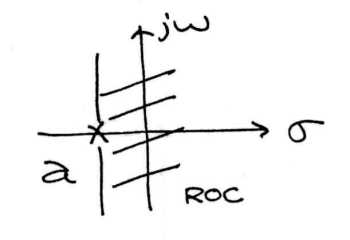 (a) The Region of Convergence for a causal signal.
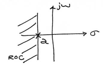 b) The Region of Convergence for an anti-causal signal.
Once we have recognized this, the natural question becomes: What do we do when we have multiple poles? The simple answer is that we take the intersection of all of the regions of convergence of the respective poles.
Example \(\PageIndex{1}\)
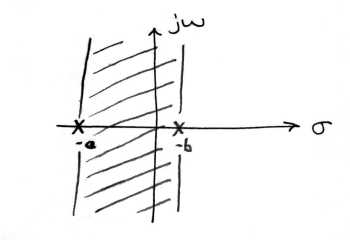
Find \(H(s)\) and state the region of convergence for \(h(t)=e^{-(a t)} u(t)+e^{-(b t)} u(-t)\)
Breaking this up into its two terms, we get transfer functions and respective regions of convergence of
\[\begin{array}{l}
H_{1}(s)=\frac{1}{s+a}, \: \operatorname{Re}(s)>-a \\
H_{2}(s)=\frac{-1}{s+b}, \: \operatorname{Re}(s)<-b
\end{array} \nonumber \]
\(-b>\operatorname{Re}(s)>-a\). If \(a>b\), we can represent this graphically. Otherwise, there will be no region of convergence.