
11.9: Continuous Time Filter Design
- Page ID
- 23172

Introduction
Analog (Continuous-Time) filters are useful for a wide variety of applications, and are especially useful in that they are very simple to build using standard, passive R,L,C components. Having a grounding in basic filter design theory can assist one in solving a wide variety of signal processing problems.
Estimating Frequency Response from Z-Plane
One of the motivating factors for analyzing the pole/zero plots is due to their relationship to the frequency response of the system. Based on the position of the poles and zeros, one can quickly determine the frequency response. This is a result of the correspondence between the frequency response and the transfer function evaluated on the unit circle in the pole/zero plots. The frequency response, or DTFT, of the system is defined as:
\[\begin{aligned}
H(w) &=\left.H(z)\right|_{z, z=e^{j w}} \\[4pt]
&=\frac{\displaystyle \sum_{k=0}^{M} b_{k} e^{-(j w k)}}{\displaystyle \sum_{k=0}^{N} a_{k} e^{-(j w k)}}
\end{aligned} \nonumber \]
Next, by factoring the transfer function into poles and zeros and multiplying the numerator and denominator by \(e^{jw}\) we arrive at the following equations:
\[H(w)=\left|\frac{b_{0}}{a_{0}}\right| \frac{\displaystyle\prod_{k=1}^{M}\left|e^{j w}-c_{k}\right|}{\displaystyle\prod_{k=1}^{N}\left|e^{j w}-d_{k}\right|} \label{11.50} \]
From Equation \ref{11.50} we have the frequency response in a form that can be used to interpret physical characteristics about the filter's frequency response. The numerator and denominator contain a product of terms of the form \(\left|e^{j w}-h\right|\), where \(h\) is either a zero, denoted by \(c_k\) or a pole, denoted by \(d_k\). Vectors are commonly used to represent the term and its parts on the complex plane. The pole or zero, \(h\), is a vector from the origin to its location anywhere on the complex plane and \(e^{jw}\) is a vector from the origin to its location on the unit circle. The vector connecting these two points, \(\left|e^{j w}-h\right|\), connects the pole or zero location to a place on the unit circle dependent on the value of \(w\). From this, we can begin to understand how the magnitude of the frequency response is a ratio of the distances to the poles and zero present in the z-plane as \(w\) goes from zero to pi. These characteristics allow us to interpret \(|H(w)|\) as follows:
\[|H(w)|=\left|\frac{b_{0}}{a_{0}}\right| \frac{\displaystyle\prod \text { "distances from zeros" }}{\displaystyle\prod \text { "distances from poles" }} \nonumber \]
In conclusion, using the distances from the unit circle to the poles and zeros, we can plot the frequency response of the system. As \(w\) goes from \(0\) to \(2 \pi\), the following two properties, taken from the above equations, specify how one should draw \(|H(w)|\).
While moving around the unit circle...
- If close to a zero, then the magnitude is small. If a zero is on the unit circle, then the frequency response is zero at that point.
- If close to a pole, then the magnitude is large. If a pole is on the unit circle, then the frequency response goes to infinity at that point.
Drawing Frequency Response from Pole/Zero Plot
Let us now look at several examples of determining the magnitude of the frequency response from the pole/zero plot of a z-transform. If you have forgotten or are unfamiliar with pole/zero plots, please refer back to the Pole/Zero Plots (Section 12.5) module.
Example \(\PageIndex{1}\)
In this first example we will take a look at the very simple z-transform shown below:
\[H(z)=z+1=1+z^{−1} \nonumber \]
\[H(w)=1+e^{−(jw)} \nonumber \]
For this example, some of the vectors represented by \(\left|e^{j w}-h\right|\), for random values of \(w\), are explicitly drawn onto the complex plane shown in the figure below. These vectors show how the amplitude of the frequency response changes as ww goes from 00 to 2π2, and also show the physical meaning of the terms in Equation \ref{11.50} above. One can see that when \(w=0\), the vector is the longest and thus the frequency response will have its largest amplitude here. As \(w\) approaches \(\pi\), the length of the vectors decrease as does the amplitude of \(|H(w)|\). Since there are no poles in the transform, there is only this one vector term rather than a ratio as seen in Equation \ref{11.50}.


Example \(\PageIndex{2}\)
For this example, a more complex transfer function is analyzed in order to represent the system's frequency response.
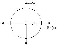
\[H(z)=\frac{z}{z-\frac{1}{2}}=\frac{1}{1-\frac{1}{2} z^{-1}} \nonumber \]
\[H(w)=\frac{1}{1-\frac{1}{2} e^{-(j w)}} \nonumber \]
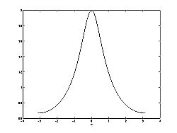
Below we can see the two figures described by the above equations. The Figure \(\PageIndex{2(a)}\) represents the basic pole/zero plot of the z-transform, \(H(w)\). Figure \(\PageIndex{2(b)}\) shows the magnitude of the frequency response. From the formulas and statements in the previous section, we can see that when \(w=0\) the frequency will peak since it is at this value of \(w\) that the pole is closest to the unit circle. The ratio from Equation \ref{11.50} helps us see the mathematics behind this conclusion and the relationship between the distances from the unit circle and the poles and zeros. As \(w\) moves from \(0\) to \(\pi\), we see how the zero begins to mask the effects of the pole and thus force the frequency response closer to \(0\).

Types of Filters
Butterworth Filters
The Butterworth filter is the simplest filter. It can be constructed out of passive R, L, C circuits. The magnitude of the transfer function for this filter is
Magnitude of Butterworth Filter Transfer Function
\[|H(j \omega)|=\frac{1}{\sqrt{1+\left(\frac{\omega}{\omega_{c}}\right)^{2 n}}} \nonumber \]
where \(n\) is the order of the filter and \(\omega_c\) is the cutoff frequency. The cutoff frequency is the frequency where the magnitude experiences a 3 dB dropoff (where \(|H(j \omega)|=\frac{1}{\sqrt{2}}\)).
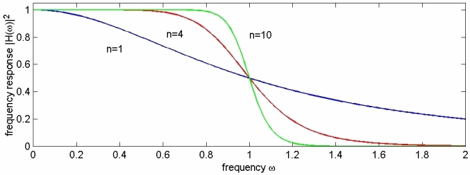
The important aspects of Figure \(\PageIndex{3}\) are that it does not ripple in the passband or stopband as other filters tend to, and that the larger nn, the sharper the cutoff (the smaller the transition band).
Butterworth filters give transfer functions \((H(j \omega)\) and \(H(s)\)) that are rational functions. They also have only poles, resulting in a transfer function of the form
\[\frac{1}{\left(s-s_{1}\right)\left(s-s_{2}\right) \cdots\left(s-s_{n}\right)} \nonumber \]
and a pole-zero plot of
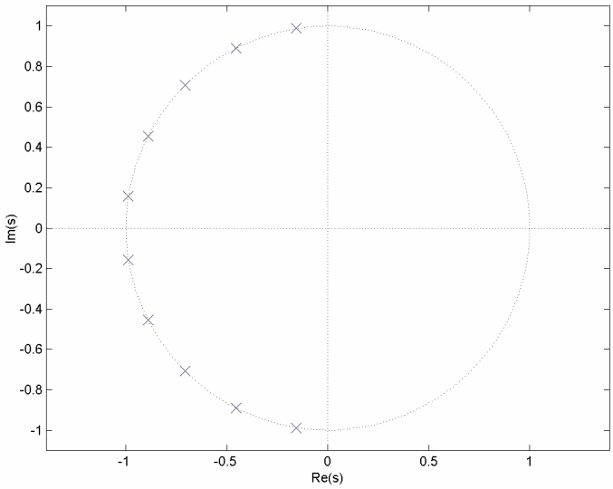
Note that the poles lie along a circle in the s-plane.
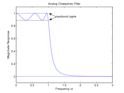
Chebyshev Filters
The Butterworth filter does not give a sufficiently good approximation across the complete passband in many cases. The Taylor's series approximation is often not suited to the way specifications are given for filters. An alternate error measure is the maximum of the absolute value of the difference between the actual filter response and the ideal. This is considered over the total passband. This is the Chebyshev error measure and was defined and applied to the FIR filter design problem. For the IIR filter, the Chebyshev error is minimized over the passband and a Taylor's series approximation at \(\omega = \infty\) is used to determine the stopband performance. This mixture of methods in the IIR case is called the Chebyshev filter, and simple design formulas result, just as for the Butterworth filter.
The design of Chebyshev filters is particularly interesting, because the results of a very elegant theory insure that constructing a frequency-response function with the proper form of equal ripple in the error will result in a minimum Chebyshev error without explicitly minimizing anything. This allows a straightforward set of design formulas to be derived which can be viewed as a generalization of the Butterworth formulas.
The form for the magnitude squared of the frequency-response function for the Chebyshev filter is
\[|F(j \omega)|^{2}=\frac{1}{1+\epsilon^{2} C_{N}(\omega)^{2}} \label{11.54} \]
where \(C_N(\omega)\) is an Nth-order Chebyshev polynomial and \(\epsilon\) is a parameter that controls the ripple size. This polynomial in \(\omega\) has very special characteristics that result in the optimality of the response function (Equation \ref{11.54}).
Bessel filters
Insert bessel filter information
Elliptic Filters
There is yet another method that has been developed that uses a Chebyshev error criterion in both the passband and the stopband. This is the fourth possible combination of Chebyshev and Taylor's series approximations in the passband and stopband. The resulting filter is called an elliptic-function filter, because elliptic functions are normally used to calculate the pole and zero locations. It is also sometimes called a Cauer filter or a rational Chebyshev filter, and it has equal ripple approximation error in both pass and stopbands.
The error criteria of the elliptic-function filter are particularly well suited to the way specifications for filters are often given. For that reason, use of the elliptic-function filter design usually gives the lowest order filter of the four classical filter design methods for a given set of specifications. Unfortunately, the design of this filter is the most complicated of the four. However, because of the efficiency of this class of filters, it is worthwhile gaining some understanding of the mathematics behind the design procedure.
This section sketches an outline of the theory of elliptic- function filter design. The details and properties of the elliptic functions themselves should simply be accepted, and attention put on understanding the overall picture. A more complete development is available in.
Because both the passband and stopband approximations are over the entire bands, a transition band between the two must be defined. Using a normalized passband edge, the bands are defined by
\[\begin{array}{c}
0<\omega<1 \quad \text { passband } \\
1<\omega<\omega_{s} \quad \text { transition band } \\
\omega_{s}<\omega<\infty \quad \text { stopband }
\end{array} \nonumber \]
This is illustrated in Figure \(\PageIndex{6}\).
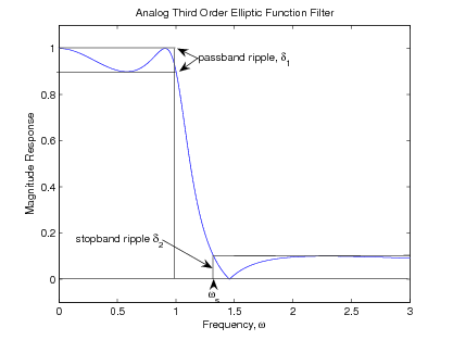
The characteristics of the elliptic function filter are best described in terms of the four parameters that specify the frequency response:
- The maximum variation or ripple in the passband \(\delta_{1}\),
- The width of the transition band \((\omega_s−1)\),
- The maximum response or ripple in the stopband \(\delta_2\), and
- The order of the filter \(N\).
The result of the design is that for any three of the parameters given, the fourth is minimum. This is a very flexible and powerful description of a filter frequency response.
The form of the frequency-response function is a generalization of that for the Chebyshev filter
\[F F(j \omega)=|F(j \omega)|^{2}=\frac{1}{1+\epsilon^{2} G^{2}(\omega)} \nonumber \]
where
\[F F(s)=F(s) F(-s) \nonumber \]
with \(F(s)\) being the prototype analog filter transfer function similar to that for the Chebyshev filter. \(G(\omega)\) is a rational function that approximates zero in the passband and infinity in the stopband. The definition of this function is a generalization of the definition of the Chebyshev polynomial.
Filter Design Demonstration
Conclusion
As can be seen, there is a large amount of information available in filter design, more than an introductory module can cover. Even for designing Discrete-time IIR filters, it is important to remember that there is a far larger body of literature for design methods for the analog signal processing world than there is for the digital. Therefore, it is often easier and more practical to implement an IIR filter using standard analog methods, and then discretize it using methods such as the Bilateral Transform.