12.9: Discrete Time Filter Design

Estimating Frequency Response from Z-Plane

One of the primary motivating factors for utilizing the z-transform and analyzing the pole/zero plots is due to their relationship to the frequency response of a discrete-time system. Based on the position of the poles and zeros, one can quickly determine the frequency response. This is a result of the correspondence between the frequency response and the transfer function evaluated on the unit circle in the pole/zero plots. The frequency response, or DTFT, of the system is defined as:

\[\begin{align}
H(w) &=\left.H(z)\right|_{z, z=e^{ j w}} \nonumber \\
&=\frac{\sum_{k=0}^{M} b_{k} e^{-(jwk)}}{\sum_{k=0}^{N} a_{k} e^{-(jw k)}}
\end{align} \nonumber \]

Next, by factoring the transfer function into poles and zeros and multiplying the numerator and denominator by \(e^{jw}\) we arrive at the following equations:

\[H(w)=\left|\frac{b_{0}}{a_{0}}\right| \frac{\prod_{k=1}^{M}\left|e^{j w}-c_{k}\right|}{\prod_{k=1}^{N}\left|e^{j w}-d_{k}\right|} \label{12.80} \]

From Equation \ref{12.80} we have the frequency response in a form that can be used to interpret physical characteristics about the filter's frequency response. The numerator and denominator contain a product of terms of the form \(|e^{jw}-h|\), where \(h\) is either a zero, denoted by \(c_k\) or a pole, denoted by \(d_k\). Vectors are commonly used to represent the term and its parts on the complex plane. The pole or zero, \(h\), is a vector from the origin to its location anywhere on the complex plane and \(e^{jw}\) is a vector from the origin to its location on the unit circle. The vector connecting these two points, \(|e^{jw}-h|\), connects the pole or zero location to a place on the unit circle dependent on the value of \(w\). From this, we can begin to understand how the magnitude of the frequency response is a ratio of the distances to the poles and zero present in the z-plane as ww goes from zero to pi. These characteristics allow us to interpret \(|H(w)|\) as follows:

\[|H(w)|=\left|\frac{b_{0}}{a_{0}}\right| \frac{\prod \text { "distances from zeros" }}{\prod \text { "distances from poles" }} \nonumber \]

Drawing Frequency Response from Pole/Zero Plot

Let us now look at several examples of determining the magnitude of the frequency response from the pole/zero plot of a z-transform. If you have forgotten or are unfamiliar with pole/zero plots, please refer back to the Pole/Zero Plots (Section 12.5) module.

Example \(\PageIndex{1}\)

In this first example we will take a look at the very simple z-transform shown below:

\[H(z)=z+1=1+z^{-1} \nonumber \]

\[H(w)=1+e^{-(j w)} \nonumber \]

For this example, some of the vectors represented by \(\left|e^{j w}-h\right|\), for random values of \(w\), are explicitly drawn onto the complex plane shown in Figure \(\PageIndex{1}\) below. These vectors show how the amplitude of the frequency response changes as \(w\) goes from \(0\) to \(2 \pi\), and also show the physical meaning of the terms in Equation \ref{12.80} above. One can see that when \(w=0\), the vector is the longest and thus the frequency response will have its largest amplitude here. As ww approaches \(\pi\), the length of the vectors decrease as does the amplitude of \(|H(w)|\). Since there are no poles in the transform, there is only this one vector term rather than a ratio as seen in Equation \ref{12.80}.

(a) Pole/Zero Plot

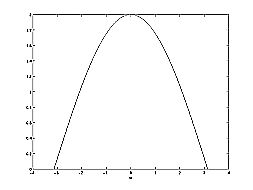
(b) Frequency Response: \(|H(w)|\)

Figure \(\PageIndex{1}\): The first figure represents the pole/zero plot with a few representative vectors graphed while the second shows the frequency response with a peak at \(+2\) and graphed between plus and minus \(\pi\).

Example \(\PageIndex{2}\)

For this example, a more complex transfer function is analyzed in order to represent the system's frequency response.

\[H(z)=\frac{z}{z-\frac{1}{2}}=\frac{1}{1-\frac{1}{2} z^{-1}} \nonumber \]

\[H(w)=\frac{1}{1-\frac{1}{2} e^{-(j w)}} \nonumber \]

Below we can see the two figures described by the above equations. The Figure \(\PageIndex{2}(a)\) represents the basic pole/zero plot of the z-transform, \(H(w)\). Figure \(\PageIndex{2}(b)\) shows the magnitude of the frequency response. From the formulas and statements in the previous section, we can see that when \(w=0\) the frequency will peak since it is at this value of ww that the pole is closest to the unit circle. The ratio from Equation \ref{12.80} helps us see the mathematics behind this conclusion and the relationship between the distances from the unit circle and the poles and zeros. As \(w\) moves from \(0\) to \(\pi\), we see how the zero begins to mask the effects of the pole and thus force the frequency response closer to \(0\).

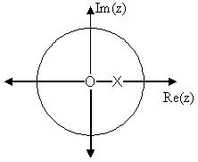
(a) Pole/Zero Plot

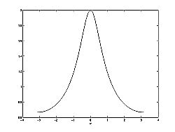
(b) Frequency Response: \(|H(w)|\)

Figure \(\PageIndex{2}\): The first figure represents the pole/zero plot while the second shows the frequency response with a peak at \(+2\) and graphed between plus and minus \(\pi\).

Interactive Filter Design Illustration

Figure \(\PageIndex{3}\): Digital filter design LabVIEW virtual instrument by NI from http://cnx.org/content/m13115/latest/.

Conclusion

In conclusion, using the distances from the unit circle to the poles and zeros, we can plot the frequency response of the system. As ww goes from \(0\) to \(2\pi\), the following two properties, taken from the above equations, specify how one should draw \(|H(w)|\).

While moving around the unit circle...

1. if close to a zero, then the magnitude is small. If a zero is on the unit circle, then the frequency response is zero at that point.
2. if close to a pole, then the magnitude is large. If a pole is on the unit circle, then the frequency response goes to infinity at that point.