
13.2: The Fast Fourier Transform (FFT)
- Page ID
- 22922

Introduction
The Fast Fourier Transform (FFT) is an efficient O(NlogN) algorithm for calculating DFTs The FFT exploits symmetries in the \(W\) matrix to take a "divide and conquer" approach. We will first discuss deriving the actual FFT algorithm, some of its implications for the DFT, and a speed comparison to drive home the importance of this powerful algorithm.
Deriving the FFT
To derive the FFT, we assume that the signal's duration is a power of two: \(N=2^l\). Consider what happens to the even-numbered and odd-numbered elements of the sequence in the DFT calculation.
\[\begin{align}S(k) &=s(0)+s(2) e^{(-j) \frac{2 \pi 2 k}{N}}+\ldots+s(N-2) e^{(-j) \frac{2 \pi(N-2) k}{N}}+s(1) e^{(-j) \frac{2 \pi k}{N}}+s(3) e^{(-j) \frac{2 \pi \times (2+1) k}{N}}+\ldots+s(N-1) e^{(-j) \frac{2 \pi(N-2+1) k}{N}} \nonumber \\ &=s(0)+s(2)e^{(-j)\frac{2\pi k}{\frac{N}{2}}} + \ldots + s(N-2)e^{(-j) \frac{2 \pi\left(\frac{N}{2}-1\right) k}{\frac{N}{2}}} +\left( s(1)+s(3) e^{(-j) \frac{2 \pi k}{\frac{N}{2}}}+\dots+s(N-1) e^{(-j) \frac{2 \pi\left(\frac{N}{2}-1\right) k}{\frac{N}{2}}}\right) e^{\frac{-(j 2 \pi k)}{N}} \end{align} \nonumber \]
Each term in square brackets has the form of a \(\frac{N}{2}\) -length DFT. The first one is a DFT of the even-numbered elements, and the second of the odd-numbered elements. The first DFT is combined with the second multiplied by the complex exponential \(e^{\frac{-(j 2\pi k)}{N}}\). The half-length transforms are each evaluated at frequency indices \(k \in\{0, \ldots, N-1\}\). Normally, the number of frequency indices in a DFT calculation range between zero and the transform length minus one. The computational advantage of the FFT comes from recognizing the periodic nature of the discrete Fourier transform. The FFT simply reuses the computations made in the half-length transforms and combines them through additions and the multiplication by \(e^{\frac{-(j 2 \pi k)}{N}}\), which is not periodic over \(\frac{N}{2}\), to rewrite the length-N DFT. Figure \(\PageIndex{1}\) illustrates this decomposition. As it stands, we now compute two length- \(\frac{N}{2}\) transforms (complexity \(2 O\left(\frac{N^{2}}{4}\right)\)), multiply one of them by the complex exponential (complexity \(O(N)\)), and add the results (complexity \(O(N)\)). At this point, the total complexity is still dominated by the half-length DFT calculations, but the proportionality coefficient has been reduced.
Now for the fun. Because \(N=2^l\), each of the half-length transforms can be reduced to two quarter-length transforms, each of these to two eighth-length ones, etc. This decomposition continues until we are left with length-2 transforms. This transform is quite simple, involving only additions. Thus, the first stage of the FFT has \(\frac{N}{2}\) length-2 transforms (see the bottom part of Figure \(\PageIndex{1}\)). Pairs of these transforms are combined by adding one to the other multiplied by a complex exponential. Each pair requires 4 additions and 4 multiplications, giving a total number of computations equaling \(8\frac{N}{4}=\frac{N}{2}\). This number of computations does not change from stage to stage. Because the number of stages, the number of times the length can be divided by two, equals \(\log_2 N\), the complexity of the FFT is \(O(N \log N)\).
Length-8 DFT decomposition
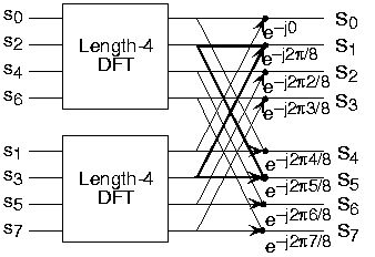 (a)
(a)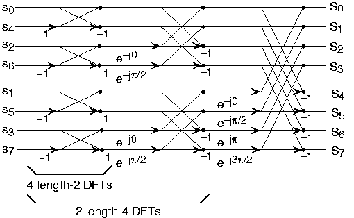 (b)
(b)Doing an example will make computational savings more obvious. Let's look at the details of a length-8 DFT. As shown on Figure \(\PageIndex{1}\), we first decompose the DFT into two length-4 DFTs, with the outputs added and subtracted together in pairs. Considering Figure \(\PageIndex{1}\) as the frequency index goes from 0 through 7, we recycle values from the length-4 DFTs into the final calculation because of the periodicity of the DFT output. Examining how pairs of outputs are collected together, we create the basic computational element known as a butterfly (Figure \(\PageIndex{2}\)).
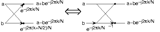
By considering together the computations involving common output frequencies from the two half-length DFTs, we see that the two complex multiplies are related to each other, and we can reduce our computational work even further. By further decomposing the length-4 DFTs into two length-2 DFTs and combining their outputs, we arrive at the diagram summarizing the length-8 fast Fourier transform (Figure \(\PageIndex{1}\)). Although most of the complex multiplies are quite simple (multiplying by \(e^{-(j\pi)}\) means negating real and imaginary parts), let's count those for purposes of evaluating the complexity as full complex multiplies. We have \(\frac{N}{2}=4\) complex multiplies and \(2N=16\) additions for each stage and \(\log_2 N=3\) stages, making the number of basic computations \(\frac{3N}{2} \log_2 N\) as predicted.
Exercise \(\PageIndex{1}\)
Note that the ordering of the input sequence in the two parts of Figure \(\PageIndex{1}\) aren't quite the same. Why not? How is the ordering determined?
- Answer
-
The upper panel has not used the FFT algorithm to compute the length-4 DFTs while the lower one has. The ordering is determined by the algorithm.
FFT and the DFT
We now have a way of computing the spectrum for an arbitrary signal: The Discrete Fourier Transform (DFT) computes the spectrum at \(N\) equally spaced frequencies from a length- \(N\) sequence. An issue that never arises in analog "computation," like that performed by a circuit, is how much work it takes to perform the signal processing operation such as filtering. In computation, this consideration translates to the number of basic computational steps required to perform the needed processing. The number of steps, known as the complexity, becomes equivalent to how long the computation takes (how long must we wait for an answer). Complexity is not so much tied to specific computers or programming languages but to how many steps are required on any computer. Thus, a procedure's stated complexity says that the time taken will be proportional to some function of the amount of data used in the computation and the amount demanded.
For example, consider the formula for the discrete Fourier transform. For each frequency we chose, we must multiply each signal value by a complex number and add together the results. For a real-valued signal, each real-times-complex multiplication requires two real multiplications, meaning we have \(2N\) multiplications to perform. To add the results together, we must keep the real and imaginary parts separate. Adding \(N\) numbers requires \(N−1\) additions. Consequently, each frequency requires \(2N+2(N−1)=4N−2\) basic computational steps. As we have \(N\) frequencies, the total number of computations is \(N(4N−2)\).
In complexity calculations, we only worry about what happens as the data lengths increase, and take the dominant term—here the \(4N^2\) term—as reflecting how much work is involved in making the computation. As multiplicative constants don't matter since we are making a "proportional to" evaluation, we find the DFT is an \(O(N^2)\) computational procedure. This notation is read "order \(N\)-squared". Thus, if we double the length of the data, we would expect that the computation time to approximately quadruple.
Exercise \(\PageIndex{2}\)
In making the complexity evaluation for the DFT, we assumed the data to be real. Three questions emerge. First of all, the spectra of such signals have conjugate symmetry, meaning that negative frequency components (\(k=\left[\frac{N}{2}+1, \ldots, N+1\right]\) in the DFT) can be computed from the corresponding positive frequency components. Does this symmetry change the DFT's complexity?
Secondly, suppose the data are complex-valued; what is the DFT's complexity now?
Finally, a less important but interesting question is suppose we want \(K\) frequency values instead of \(N\); now what is the complexity?
- Answer
-
When the signal is real-valued, we may only need half the spectral values, but the complexity remains unchanged. If the data are complex-valued, which demands retaining all frequency values, the complexity is again the same. When only \(K\) frequencies are needed, the complexity is \(O(KN)\).
Speed Comparison
How much better is \(O(N \log N)\) than \(O( N^2)\)?
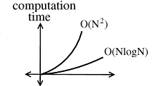
| \(N\) | \(10\) | \(100\) | \(1000\) | \(10^6\) | \(10^9\) |
|---|---|---|---|---|---|
| \(N^2\) | \(100\) | \(10^4\) | \(10^6\) | \(10^{12}\) | \(10^{18}\) |
| \(N \log N\) | \(1\) | \(200\) | \(3000\) | \(6 \times 10^6\) | \(9 \times 10^9\) |
Say you have a 1 MFLOP machine (a million "floating point" operations per second). Let \(N\) =1 million=\(10^6\).
An \(O( N^2)\) algorithm takes \(10^{12}\) Flors → \(10^6\) seconds ≃ 11.5 days.
An \(O( N \log N)\) algorithm takes \(6 \times 10^6\) Flors → 6 seconds.
Note
N = 1 million is not unreasonable.
Example \(\PageIndex{1}\)
3 megapixel digital camera spits out \(3 \times 10^6\) numbers for each picture. So for two \(N\) point sequences \(f[n]\) and \(h[n]\). If computing \(f[n]⊛h[n]\) directly: \(O( N^2)\) operations.
taking FFTs -- \(O(N \log N)\)
multiplying FFTs -- \(O(N)\)
inverse FFTs -- \(O(N \log N)\).
the total complexity is \(O(N \log N)\).
Conclusion
Other "fast" algorithms have been discovered, most of which make use of how many common factors the transform length N has. In number theory, the number of prime factors a given integer has measures how composite it is. The numbers 16 and 81 are highly composite (equaling \(2^4\) and \(3^4\) respectively), the number 18 is less so ( \(2^1 3^2\) ), and 17 not at all (it's prime). In over thirty years of Fourier transform algorithm development, the original Cooley-Tukey algorithm is far and away the most frequently used. It is so computationally efficient that power-of-two transform lengths are frequently used regardless of what the actual length of the data. It is even well established that the FFT, alongside the digital computer, were almost completely responsible for the "explosion" of DSP in the 60's.