
6.5: Continuous Time Circular Convolution and the CTFS
- Page ID
- 22876

Introduction
This module relates circular convolution of periodic signals in the time domain to multiplication in the frequency domain.
Signal Circular Convolution
Given a signal \(f(t)\) with Fourier coefficients \(c_n\) and a signal \(g(t)\) with Fourier coefficients \(d_n\), we can define a new signal, \(v(t)\), where \(v(t)=f(t) \circledast g(t)\). We find that the Fourier Series representation of \(v(t)\), \(a_n\), is such that \(a_n=c_nd_n\). \(f(t) \circledast g(t)\) is the circular convolution (Section 7.5) of two periodic signals and is equivalent to the convolution over one interval, i.e. \(f(t) \circledast g(t)=\int_{0}^{T} \int_{0}^{T} f(\tau) g(t-\tau) d \tau d t\).
Note
Circular convolution in the time domain is equivalent to multiplication of the Fourier coefficients.
This is proved as follows
\[\begin{align}
a_{n} &=\frac{1}{T} \int_{0}^{T} v(t) e^{-\left(j \omega_{0} n t\right)} \mathrm{d} t \nonumber \\
&=\frac{1}{T^{2}} \int_{0}^{T} \int_{0}^{T} f(\tau) g(t-\tau) \mathrm{d} \tau e^{-\left(\omega j_{0} n t\right)} \mathrm{d} t \nonumber \\
&=\frac{1}{T} \int_{0}^{T} f(\tau)\left(\frac{1}{T} \int_{0}^{T} g(t-\tau) e^{-\left(j \omega_{0} n t\right)} \mathrm{d} t\right) \mathrm{d} \tau \nonumber \\
&=\forall \nu, \nu=t-\tau:\left(\frac{1}{T} \int_{0}^{T} f(\tau)\left(\frac{1}{T} \int_{-\tau}^{T-\tau} g(\nu) e^{-\left(j \omega_{0}(\nu+\tau)\right)} \mathrm{d} \nu\right) \mathrm{d} \tau\right) \nonumber \\
&=\frac{1}{T} \int_{0}^{T} f(\tau)\left(\frac{1}{T} \int_{-\tau}^{T-\tau} g(\nu) e^{-\left(j \omega_{0} n \nu\right)} \mathrm{d} \nu\right) e^{-\left(j \omega_{0} n \tau\right)} \mathrm{d} \tau \nonumber \\
&=\frac{1}{T} \int_{0}^{T} f(\tau) d_{n} e^{-\left(j \omega_{0} n \tau\right)} \mathrm{d} \tau \nonumber \\
&=d_{n}\left(\frac{1}{T} \int_{0}^{T} f(\tau) e^{-\left(j \omega_{0} n \tau\right)} \mathrm{d} \tau\right) \nonumber \\
&=c_{n} d_{n}
\end{align} \nonumber \]
Exercise
Take a look at a square pulse with a period of \(T\).
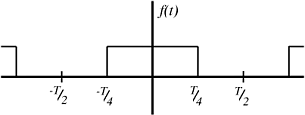
Figure \(\PageIndex{1}\)
For this signal
\[c_{n}=\left\{\begin{array}{l}
\frac{1}{T} \text { if } n=0 \\
\frac{1}{2} \frac{\sin \left(\frac{\pi}{2} n\right)}{\frac{\pi}{2} n} \text { otherwise }
\end{array}\right. \nonumber \]
Take a look at a triangle pulse train with a period of \(T\).
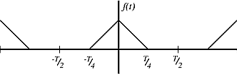
Figure \(\PageIndex{2}\)
This signal is created by circularly convolving the square pulse with itself. The Fourier coefficients for this signal are \(a_{n}=c_{n}^{2}=\frac{1}{4} \frac{\sin ^{2}}{\left(\frac{\pi}{2} n\right)}\).
Exercise \(\PageIndex{1}\)
Find the Fourier coefficients of the signal that is created when the square pulse and the triangle pulse are convolved.
- Answer
-
\(a_{n}=\left\{\begin{array}{ll}
\text { undefined } & n=0 \\
\frac{1}{8} \frac{\sin ^{3}\left(\frac{\pi}{2} n\right)}{\left(\frac{\pi}{2} n\right)^{3}} & \text { otherwise }
\end{array}\right.\)
Conclusion
Circular convolution in the time domain is equivalent to multiplication of the Fourier coefficients in the frequency domain.