7.3: Common Discrete Fourier Series

Introduction

Once one has obtained a solid understanding of the fundamentals of Fourier series analysis and the General Derivation of the Fourier Coefficients, it is useful to have an understanding of the common signals used in Fourier Series Signal Approximation.

Deriving the Coefficients

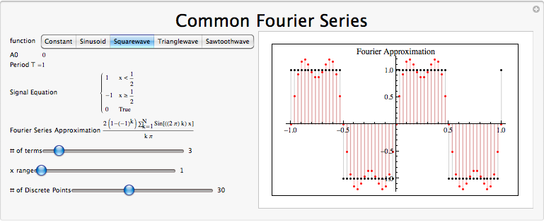
Consider a square wave \(f(x)\) of length 1. Over the range [0,1), this can be written as

\[x(t)=\left\{\begin{array}{rl}
1 & t \leq \frac{1}{2} \\
-1 & t>\frac{1}{2}
\end{array}\right. \nonumber \]

Fourier series approximation of a square wave

Figure \(\PageIndex{1}\): Fourier series approximation to \(sq(t)\). The number of terms in the Fourier sum is indicated in each plot, and the square wave is shown as a dashed line over two periods.

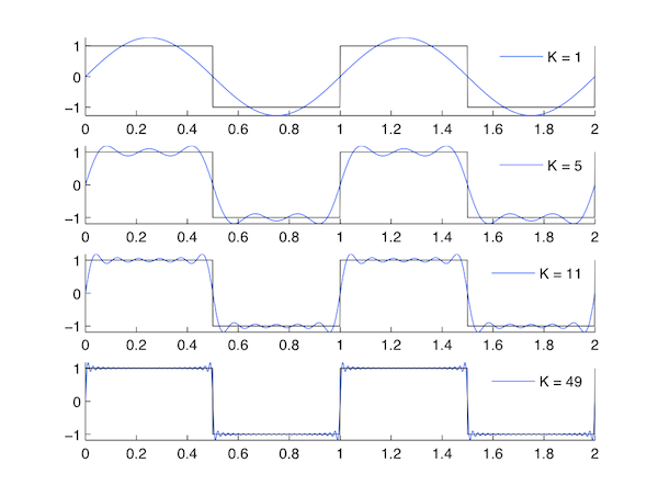
Real Even SignalsGiven that the square wave is a real and even signal,

• \(f(t)=f(−t)\) EVEN
• \(f(t)=f^*(t)\) REAL

therefore,

• \(c_n=c_{−n}\) EVEN
• \(c_n=c_n^*\) REAL

Deriving the Coefficients for other signals

The Square wave is the standard example, but other important signals are also useful to analyze, and these are included here.

Constant Waveform

This signal is relatively self-explanatory: the time-varying portion of the Fourier Coefficient is taken out, and we are left simply with a constant function over all time.

\[x(t)=1 \nonumber \]

Fourier series approximation of a constant wave

Figure \(\PageIndex{2}\)

Sinusoid Waveform

With this signal, only a specific frequency of time-varying Coefficient is chosen (given that the Fourier Series equation includes a sine wave, this is intuitive), and all others are filtered out, and this single time-varying coefficient will exactly match the desired signal.

\[x(t)=\cos (2 \pi t) \nonumber \]

Fourier series approximation of a sinusoid wave

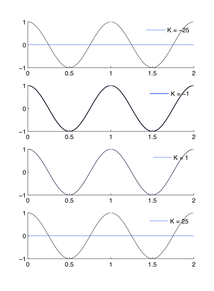
Figure \(\PageIndex{3}\)

Triangle Waveform

\[x(t)=\left\{\begin{array}{rl}
t & t \leq 1 / 2 \\
1-t & t>1 / 2
\end{array}\right. \nonumber \]

This is a more complex form of signal approximation to the square wave. Because of the Symmetry Properties of the Fourier Series, the triangle wave is a real and odd signal, as opposed to the real and even square wave signal. This means that

• \(f(t)=−f(−t)\) ODD
• \(f(t)=f^*(t)\) REAL

therefore,

• \(c_n=−c_{−n}\)
• \(c_n=−c_n^*\) IMAGINARY

Fourier series approximation of a triangle wave

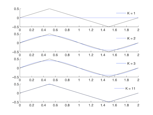
Figure \(\PageIndex{4}\)

Sawtooth Waveform

\[x(t) = t/2 \nonumber \]

Because of the Symmetry Properties of the Fourier Series, the sawtooth wave can be defined as a real and odd signal, as opposed to the real and even square wave signal. This has important implications for the Fourier Coefficients.

Fourier series approximation of a sawtooth wave

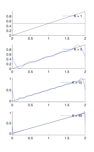
Figure \(\PageIndex{5}\)

DFT Signal Approximation

Figure \(\PageIndex{6}\): Interact (when online) with a Mathematica CDF demonstrating the common Discrete Fourier Series. To download, right-click and save as .cdf.

Conclusion

To summarize, a great deal of variety exists among the common Fourier Transforms. A summary table is provided here with the essential information.

Table \(\PageIndex{1}\): Common Discrete Fourier Transforms

Description	Time Domain Signal for \(n \in \mathbb{Z}[0, N-1]\)	Frequency Domain Signal \(k \in \mathbb{Z}[0, N-1]\)
Constant Function	1	\(\delta(k)\)
Unit Impulse	\(\delta(n)\)	\(\frac{1}{N}\)
Complex Exponential	\(e^{j 2 \pi m n / N}\)	\(\delta\left((k-m)_{N}\right)\)
Sinusoid Waveform	\(\cos (j 2 \pi m n / N)\)	\(\frac{1}{2}\left(\delta\left((k-m)_{N}\right)+\delta\left((k+m)_{N}\right)\right)\)
Box Waveform \((M < N/2)\)	\(\delta(n)+\sum_{m=1}^{M} \delta\left((n-m)_{N}\right)+\delta\left((n+m)_{N}\right)\)	\(\frac{\sin ((2 M+1) k \pi / N)}{N \sin (k \pi / N)}\)
Dsinc Waveform \((M<N/2)\)	\(\frac{\sin ((2 M+1) n \pi / N)}{\sin (n \pi / N)}\)	\(\delta(k)+\sum_{m=1}^{M} \delta\left((k-m)_{N}\right)+\delta((k+m)_N)\)