
9.4: PID tuning via Frequency Responses with Bode Plots
- Page ID
- 22415

Description of Amplitude Ratio, Phase Shift and Frequency Response
A good way to understand the physical meaning of amplitude ratio and phase shift and how they change as a function of the frequency of the input stream is through the analysis of a simple system. A well-insulated continuously-stirred tank reactor (CSTR) with an input flow equal to its output flow is a good example (Figure \(\PageIndex{1}\)). For this description we consider inlet and outlet temperature, but inlet concentration or feed rate could also be used.

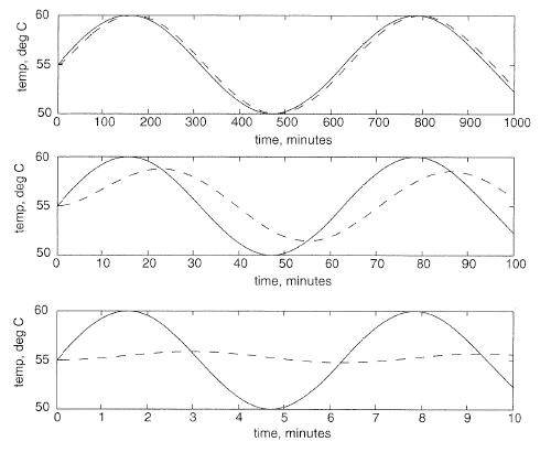
If the CSTR is initially at 55˚C, and the inlet flow has a temperature that fluctuates sinusoidally between 50˚C and 60˚C, the outlet temperature will also vary sinusoidally. If the fluid has a large residence time in the tank, and the frequency of the temperature variation of the input fluid is high relative to the residence time. Then the outlet temperature will also vary quickly in a sinusoidal fashion, but with a significantly smaller amplitude than that of the inlet. The large hold up in the well mixed tank dampens the fluctuations in the inlet temperature. In contrast, if the the frequency of the inlet temperature sine wave is low relative to the fluid residence time, the output will also be a sine wave with temperatures ranging from 50˚C to 60˚C.
In both cases described above there will be a lag or phase shift between the input and the output of the system (see the figure immediately below). In our example, the phase shift is controlled by the average residence time of fluid in the tank. The time constant of this system is the average residence time of the tank. A system with a small residence time will respond very quickly to changes in input flow rate, and large residence times will result in sizable lag time.
As frequency of the temperature variation increases, the period of the input decreases and the phase shift becomes larger. This can be seen in Figure \(\PageIndex{2}\):
Imagine that we have a sensitive reaction that must be maintained with 3˚C of 55˚C, it now becomes of utmost importance that we understand the frequency response of this CSTR system. Here in lies the utility of Bode plots; they depict a range of different frequency responses in two plots. This allows a relatively rapid determination of system robustness. In addition, frequency response and Bode plot analysis can be used to tune PID control systems.
Frequency Response
For a given process described by \(Y(t)=\hat{G} X(t)\), one considers a sinusoidal input
\[X(t)=\sin (\omega t)\nonumber \]
After a long time, the solution will also be sinusoidal, with
\[Y(t) \sim A R \sin (\omega t+\phi)\nonumber \]
where \(AR\) is the amplitude ratio (must be a positive number) and \(\phi\)is the phase lag (\(\phi < 0\)) or phase lead (\(\phi > 0\)).
Sometimes, to solve for \(Y(t)\) using an ODE solver, it is useful to have the process equation in the form \(X(t)=\hat{G}^{-1} Y(t)\) and define \(\hat{G}^{-1}\) instead of \(\hat{G}\).
Expressions for AR and \(\phi\)
First-Order System
\[A R=\frac{1}{\sqrt{1+\omega^{2} \tau_{p}^{2}}}\nonumber \]
\[\phi=\tan ^{-1}\left(-\omega \tau_{p}\right)\nonumber \]
Second-Order System
\[A R=\frac{1}{\sqrt{\left(1-\omega^{2} \tau_{p}^{2}\right)^{2}+\left(2 \zeta \omega \tau_{p}\right)^{2}}}\nonumber \]
\[\phi=\tan ^{-1}\left(\frac{-2 \zeta_{p} \omega \tau_{p}}{1-\omega^{2} \tau_{p}^{2}}\right)\nonumber \]
Dead Time

\[A R=1]
\[\phi=-\omega \tau_{\text {dead}}\nonumber \]
Systems in series
\[A R=A R_{1} \cdot A R_{2} \cdot \ldots\nonumber \]
\[\log A R=\log A R_{1}+\log A R_{2}+\ldots\nonumber \]
\[\phi=\phi_{1}+\phi_{2}+\ldots\nonumber \]
P Controller
\[\hat{G}_{c}=K_{c}\nonumber \]
\[A R=K_{c}\nonumber \]
\[\phi=0\nonumber \]
PI Controller
\[\hat{G}_{c}=K_{c}\left(1+\frac{1}{\tau_{I}} \int_{0}^{t} d t^{\prime}\right)\nonumber \]
\[\phi=\tan ^{-1}\left(-\frac{1}{\omega \tau_{I}}\right)\nonumber \]
PD Controller
\[A R=K_{c} \sqrt{1+\omega^{2} \tau_{D}^{2}}\nonumber \]
\[\phi=\tan ^{-1}\left(\omega \tau_{D}\right)\nonumber \]
PID Controller
\[\phi=\tan ^{-1}\left(\omega \tau_{D}-\frac{1}{\omega \tau_{I}}\right)\nonumber \]
Introduction to Bode Plots
Because it’s impossible to perfectly model a real chemical process, control engineers are interested in characterizing the robustness of the system – that is, they want to tune controllers to withstand a reasonable range of change in process parameters while maintaining a stable feedback system. Bode plots provide an effective means to quantify the system’s stability. Bode plots describe an open or closed-loop system as a function of input frequency and give a picture of the system’s stability. If all inputs into a system were constant, it would be a relatively simple task to control the system and its output. However, if an input value, such as temperature, varies sinusoidally, then the output should also be describable as a sinusoidal function. In this case Bode plots are a useful tool for predicting the response of the system. There are two Bode plots used to describe a system. The first shows amplitude ratio as a function of frequency. The amplitude ratio is the amplitude of the output sine wave divided by the input sine wave. The second plot graphs phase shift as a function of frequency, where phase shift is the time lag between the output and the input sine curves divided by the period of either of the sine curves and then multiplied by -360° (or \(-2π\) radians) to express this shift as an angle.
Constructing Bode Plots
Bode plots concisely display all relevant frequency input and output information on two plots: amplitude ratio as a functions of frequency and phase shift as a function of frequency. The amplitude ratio plot is a log-log plot while the phase angle plot is a semilog (or log-linear) plot.
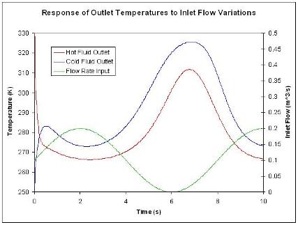
To construct a Bode plot, an engineer would have empirical data showing input and output values that vary as sinusoidal functions of time. For instance, there might be inlet temperature data that varies sinusoidally and the outlet temperature data that also varies sinusoidally. For example, given a heat exchanger that is used to cool a hot stream, we can vary the flow rate of the hot stream and model it sinusodially. (This can be done using ODEs & an Excel model of a heat exchanger.)
Figure \(\PageIndex{3}\) includes inlet flowrate (process fluid stream) varying as a sinusoidal function and the hot temperature exiting the heat exchanger likewise varying as a sinusoidal function. Portions of this graph are not yet at steady-state.
Bode plots are constructed from steady-state data. Figure \(\PageIndex{4}\) shows part of the steady-state region of the same data used for Figure \(\PageIndex{3}\).
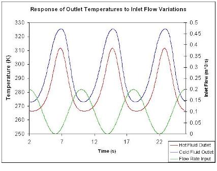
To collect a single data point for a Bode plot we will use the information from a single period of the inlet flow rate and the corresponding temperature from the hot exiting stream.
The amplitude ratio, \(AR\), is the ratio of the amplitude of the output sinusoidal curve divided by the amplitude of the input sinusoidal curve.
\[A R=\dfrac{\text { output amplitude }}{\text {input amplitude}} \nonumber \nonumber \]
The value of the amplitude ratio should be unitless so if the units of the input frequency and the units of the output frequency are not the same, the frequency data should first be normalized. For example, if the input frequency is in ˚C/min and the output frequency is also in ˚C/min, then AR is unitless and does not need to be normalized. If, instead, the input frequency is in L/min and the output frequency is in ˚C/min, then AR = ˚C/liters. In this case the inlet and outlet frequencies need to be normalized because the ratio AR = ˚C/L doesn’t say anything about the physical meaning of the system. The value of AR would be completely different if the units of AR were Kelvin/gal.
To find the phase shift, the periods of the input and output sine curves need to be found. Recall that the period, \(P\), is the length of time from one peak to the next.
\[P=\frac{1}{f}=\frac{2 \pi}{\omega}\nonumber \]
with \(f\) is the frequency and \(\omega\) is the angular frequency (rad/sec)
The phase shift is then found by
\[\phi=-2 \pi \left(\dfrac{\Delta P}{P}\right)\nonumber \]
Using these values found from multiple perturbations in feed flow rate it is possible to construct the following Bode plots:
Rules of Thumb when analyzing Bode plots
Generally speaking, a gain change shifts the amplitude ratio up or down, but does not affect the phase angle. A change in the time delay affects the phase angle, but not the amplitude ratio. For example, an increase in the time delay makes the phase shift more negative for any given frequency. A change in the time constant changes both the amplitude ratio and the phase angle. For example, an increase in the time constant will decrease the amplitude ratio and make the phase lag more negative at any given frequency.
| Change | Effect |
|---|---|
| Gain Change | Amplitude ratio is shifted up or down; no change in phase angle |
| Time Delay | Phase angle changes, but no change in amplitude ratio |
Prior to the advent of powerful computer modeling tools, controls engineers would model systems using transfer functions. Readers interested in learning more about how these were used to construct Bode plots should refer to Bequette's Process Control: Modeling, Design, and Simulation (see References). This wiki assumes that the engineer already has data in Excel, etc, that shows the sinusoidal behavior of input and outputs.
Bode Stability Criterion
A control system is unstable if the open-loop frequency response exhibits an AR exceeding unity at the frequency for which the phase lag is 180 degrees. This frequency is called the crossover frequency. Adjusting the gain so that the AR < 1 for - phi < (180 minus phase margin) results in acceptable stability if the phase margin is greater than 30 degrees.
As previously mentioned, the controls engineer uses Bode plots to characterize the stability of the system. If you were to find that the amplitude ratio is greater than 1 the system would be unstable at that frequency. An important stability criterion is that AR < 1 when phase shift = -180 degrees (or -pi radians). This is called the Bode stability criterion and if it holds for a closed-loop system, then that system will be stable. If this criterion is not satisfied and you were to put a feedback controller on this process, as done in PID tuning via optimization, the process would explode due to the response lag. The reason for this is that the system might think temperature is too low when it's actually to high, so it would decrease cooling water rather than increase it. Also, with an AR < 1, an error in input is amplified in the output, so the system will lose control due to amplification of error. This could obviously be a dangerous situation, for example in an exothermic CSTR, which could explode.
Frequency Response in Mathematica
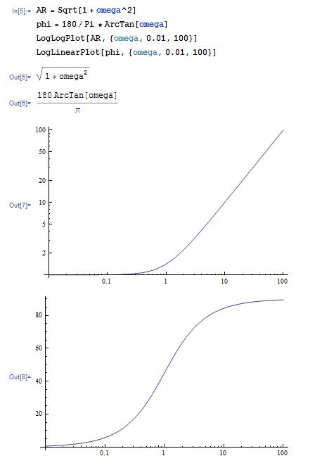
Bode plot for PD controller, ΤD = 1:
AR = Sqrt[1 + omega^2]
phi = 180/Pi*ArcTan[omega]
LogLogPlot[AR,{omega,0.01,100}]
LogLinearPlot[phi,{omega,0.01,100}]
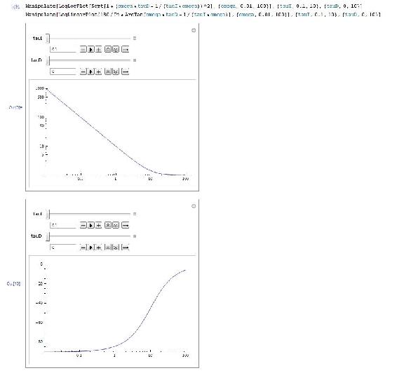
Bode plot for PID controller, using the \Manipulate" function to watch the effect of varying the values of both Tau_I and Tau_D:
Manipulate[LogLogPlot[Sqrt[1 + (omega*tauD - 1/(tauI*omega))^2],{omega,0.01,100}],{tauI,0.1,10},{tauD,0,10}]
Manipulate[LogLinearPlot[180/Pi*ArcTan[omega*tauD - 1/(tauI*omega)],{omega,0.01,100}],{tauI,0.1,10},{tauD,0,10}]
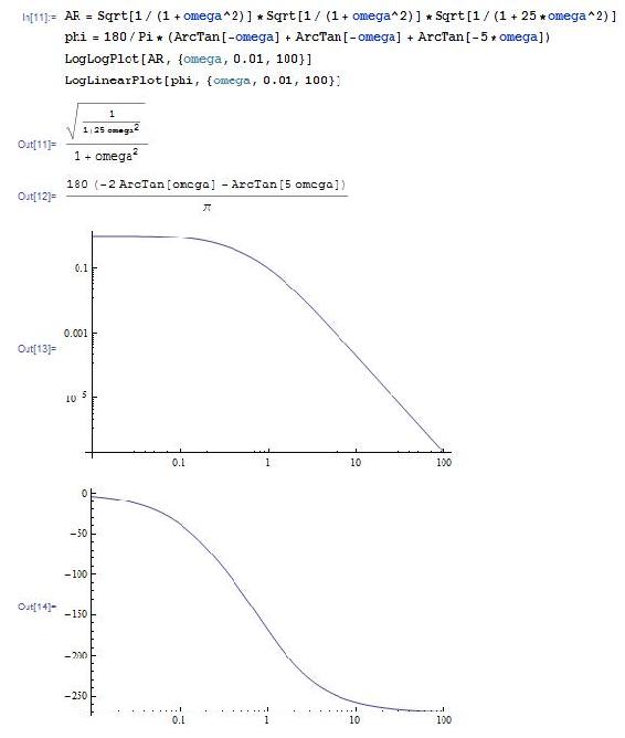
Bode plot for open-loop operation of third-order system with a P controller:
AR = Sqrt[1/(1+omega^2)]*Sqrt[1/(1+omega^2)]*Sqrt[1/(1+25*omega ^ 2)] phi = 180/Pi*(ArcTan[-omega] + ArcTan[-omega] + ArcTan[-5*omega]) LogLogPlot[AR,{omega,0.01,100}] LogLinearPlot[phi,{omega,0.01,100}]
Find crossover frequency:
FindRoot[phi==-180,{omega,1}]
This yields omega = 1.18322 which is the crossover frequency, and can be used to determine the amplitude ratio (ask mathematica for AR) the gain (Kc=1/AR)
To determine what the gain should be set to at a phase margin of 30 degrees (safe operating conditions) use the following in mathematica:
FindRoot[phi==-150,{omega,1}]
The phase margin of Cohen-Coon and other frequency analysis (such as Zielger-Nicholas) can be calculated by using the gain (Kc) value gotten from the method a typing the following into mathematica:
NSolve[Kc*AR==1,omega]
Derivations
Assume a first-order process with input \(X(t)\), output \(Y(t)\), and operator
\[\hat{G}^{-1}=\left(\tau \frac{\delta}{\delta t}+1\right)\nonumber \]
where
\[X(t)=\hat{G}^{-1} Y(t)=\left(\tau \frac{\delta}{\delta t}+1\right) Y(t)=\tau Y^{\prime}(t)+Y(t) \label{1} \]
For Bode Plot Analysis, we assume a periodic input to the system:
\[X(t) = \sin(ωt)\nonumber \]
Based on this input, we can hypothesize that:
\[Y(t) = AR * \sin(ωt + φ)\nonumber \]
From this hypothesis, we can replace Equation \ref{1} with our functions for \(X(t)\) and \(Y(t)\). This is shown below.
\[X(t) = \tau Y'(t) + Y(t) \label{1a} \]
\[\begin{align} \sin (\omega t) &=\tau \frac{\delta}{\delta t}(A R \sin (\omega t+\phi))+A R \sin (\omega t+\phi) \label{2} \\[4pt] &= AR(τω \cos(ωt + φ)) + \sin(ωt + φ) \label{3} \end{align} \]
Using trigonometric identities, we can replace \(\cos(ωt + φ)\) with \(\cos(ωt)cos(φ) − \sin(ωt)sin(φ)\) and \(\sin(ωt + φ)\) with \(\sin(ωt)cos(φ) + \cos(ωt)sin(φ)\) to get:
\[\sin (\omega t)=A R(\omega T(\cos (\omega t) \cos (\varphi)-\sin (\omega t) \sin (\varphi))+\sin (\omega t) \cos (\varphi)+\cos (\omega t) \sin (\varphi)) \label{4a} \]
To solve for \(AR\) and \(φ\), we can match the coefficients for the \(\sin(ωt)\) term and \(\cos(ωt)\) term on the left and right side of Equation \ref{4a}.
Coefficient of \(\cos(ωt)\):
\[0 = AR(ωτ\cos(φ) + \sin(φ)) \label{5} \]
Coefficient of \(\sin(ωt)\):
\[1 = AR( − ωτ\sin(φ) + \cos(φ)) \label{6} \]
From Equation \ref{5}, we can divide both sides by \(AR\cos(φ)\) and rearranging to get:
\[\tan (\phi)=-\omega \tau \label{7a} \]
or
\[\phi=\tan^{-1}(-\omega \tau) \label{7b} \]
Based on this relationship, we can draw a triangle with the angle \(φ\) and the relationship shown in Equation \ref{7b}. A picture of the triangle is shown below.
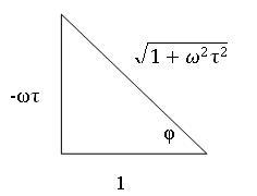
From Equation \ref{6} and the triangle above, we can solve for AR:
\[\begin{align} AR &=\frac{1}{-\omega \tau(\sin (\phi))+\cos (\phi)} \\[4pt] &=\frac{1}{-\omega \tau\left(\frac{-\omega \tau}{\sqrt{1+\omega^{2} \tau^{2}}}\right)+\frac{1}{\sqrt{1+\omega^{2} \tau^{2}}}} \\[4pt] &=\frac{1}{\sqrt{1+\omega^{2} \tau^{2}}} \label{8} \end{align} \]
Determining Stable Controller Gain and Phase Margin
Tuning via phase margin is a more precise method than tuning through Cohen-Coon Rule and Ziegler-Nichols Tuning Rule. We can find the gain and phase margin by using bode plots or by an analytical method.
To find a safe controller gain, use the following steps:
- Construct Bode Plot of \(\log AR\) versus \(\log ωτ\) and \(φ\) versus \(\log ωτ\)
- Use the above plot to find \(ωτ\) such that \(φ = -180^o + φ_{PM}\).
- Use \(ωτ\) found from above step to find \(AR\) in \(\log AR\) versus \(\log ωτ\) plot.
- \(K_{C s a f e}=\frac{1}{A R}\)
To find the phase margin, use the following steps:
- Construct Bode Plot of LogAR versus Log ωτ and φ versus Log ωτ
- Use the above plot to find ωτ such that AR=1.
- Use ωτ found from above step to find φ in φ versus Log ωτ plot.
- φPM = 180 − | φAR = 1 |
Finding the gain with a phase margin:
- Use your expression for Φ, set Φ to the desired value and find the root for ω.
- Input the value obtained for ω in your expression for AR.
- \(K_{C}=\frac{1}{A R}\)
Finding the phase margin with a gain:
- Use your expression for AR, set
 and solve for ω.
 - Input the value obtained for ω in your expression for Φ.
Determining the Slope of a Bode Plot
Sometimes it is necessary to determine the relative shape of a Bode Plot without the use of a computer or ODE equation solver. In sketching the relative shape, there are three main parts of a basic Bode Plot that must be considered.
- Crossing point
- Starting value
- Slope
Crossing Point
The crossing point of the Bode Plot is when the frequency, ω, is equal to 1 / τ . If the x-axis of the Bode Plot is ωτ, the crossing point will be at x-axis = 1. If there are multiple values of τ, there may be multiple crossing points, each at the frequency where ω is equal to 1 / τ . If there are multiple τ values, and the x-axis is ωτ, it must be specified which τ the x-axis is referring to.
Starting Value
The starting value depends on the \(K_C\) and \(K_P\) values contributing to the process.
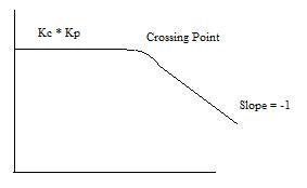
Slope
The slope for an uncontrolled process is equal to the negative of the order of the process. For example, if there is a first-order process with no controller the slope of the Bode Plot would be -1 (-1 for first order), after the crossing point has been reached. A picture of this Bode Plot is shown below.
For a process controlled by a PD controller, the AR is essentially the inverse of the first-order system AR, meaning that the slope addition from a PD controller is a +1, instead of a -1 as in a first-order process. For a second-order system with a PD controller the final slope will be -1 (-2 from the second order process, +1 from PD). However, there may be multiple crossing points, whose location depends on the value of τP and τD. Remember that the crossing point is where ωτ equals one. Since the slope contribution only comes after the crossing point, a Bode Plot for τD less than τP would look like the picture below.
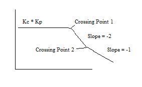
- Crossing point 1 is where ωτP is 1 and crossing point 2 is where ωτD is 1.
- Similarly, if τD is greater than τ, the slope would first go to +1, then to -1.
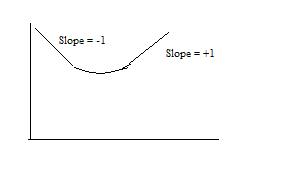
For a PI controller, the slope contribution from the controller comes before the crossing point, and then goes to zero after the crossing point. A PID controller would therefore look like the picture shown below, assuming τD = τI .
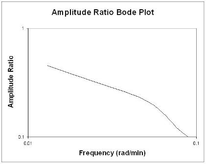
You are a controls engineer and wish to characterize a heat exchanger used in a chemical process. One of the many things you are interested in knowing about the system is how the hot outlet temperature responds to fluctuations in the inlet flow rate. Using data for a particular inlet flow rate, you graphed normalized (why?) flow rate and normalized hot outlet temperature vs. frequency (rad/min). Use this graph to determine the amplitude ratio.
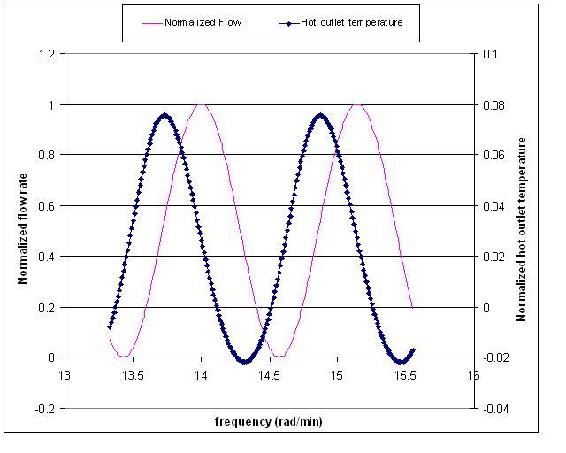
Solution
Because flow rate units and temperature do not have the same units, these values needed to be normalized before calculating the amplitude ratio. To normalize flow, use the following equation:
\[\text {F}_\text{norm}=\frac{F-\text {Fmin}}{\text {Fmax}-\text {Fmin}} \nonumber \nonumber \]
where \(F\) is the flow rate of a particular data point.
In this problem temperature, \(T\), is in ˚C, so
\[\text {Tnorm}=\frac{T-273.15}{100} \nonumber \nonumber \]
To find the amplitude of both wave functions, first recall that the amplitude of a wave is the maximum height of a wave crest (or depth of a trough). For one steady-state wave produced from a column of values in Excel, you could quickly calculate the amplitude by using the max( ) and min( ) Excel functions. [This can be found using Excel help.] If you opted to find the amplitude this way, then the amplitude for a single wave function would be
\[\text {Amplitude}=\frac{[\max ()-\min ()]}{2} \nonumber \nonumber \]
Note that this is just one way to find the amplitude of a wave. It could also be found simply by reading the values off the graph of a wave.
Once the amplitudes of the inlet and outlet waves are found, use the values to find the amplitude ratio, AR, as follows:
\[AR=\frac{\text { outlet streams amplitude }}{\text {inlet streams amplitude}}=\frac{0.0486}{0.499}=0.0974\nonumber \]
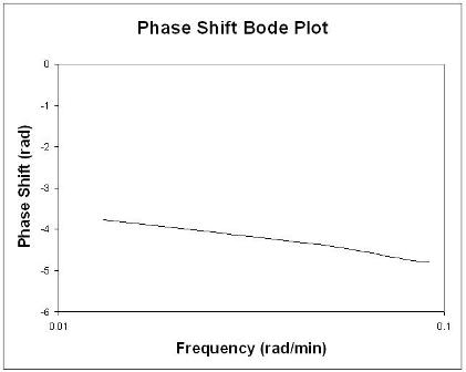
The following graph shows how inlet flow and both the hot and cold outlet temperatures vary as sinusoidal functions of time. This graph was generated using the same data for the heat exchanger of Example 1. Use this graph to find the phase shift between the inlet flow and the hot outlet stream.
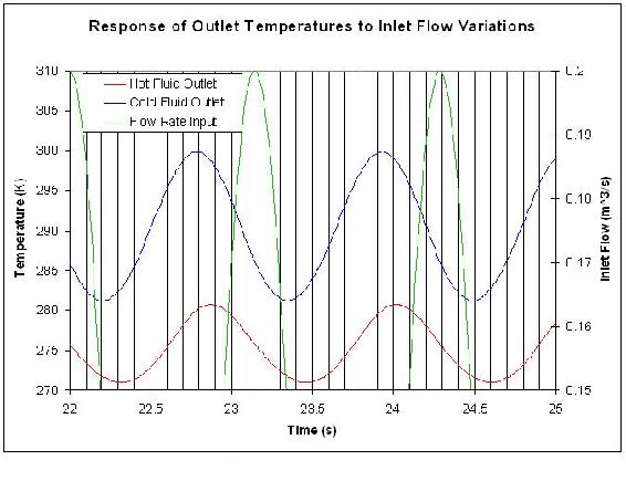
Solution
Determine the period (P) – This can be done by finding the time from one peak to the next of a given wave. In this case, we want to know the period of the inlet flow rate, so \(P = 1.14\,s\).
Determine the lag (delta P) – This can be done by finding the time difference between the peak of the inlet flow rate and the peak of the hot outlet stream. (Remember that the hot outlet wave lags the wave of the inlet flowrate).
\(\delta P = 0.87s\)
\[\text {Phaseshift}=\frac{0.87\, s}{1.14\, s} *-2 \pi=-4.80\nonumber \]
Since we're only concerned with time values for finding the phase shift, the data doesn't need to be normalized.
References
- Bequette, B. Wayne. Process Control: Modeling, Design, and Simulation. pp 172-178, 214-235. Upper Saddle River, N.J. Prentice Hall, PTR 2003.
- Liptak, Bela G. Process Control and Optimization. Volume 2. Instrument Engineers Handbook. Fourth Edition. CRC Press, Boca Raton Fl. 2003. Insertformulahere
Contributors and Attributions
- written by: Tony Martus, Kegan Lovelace, Daniel Patrick, Merrick Miranda, Jennifer DeHeck, Chris Bauman, Evan Leonard
- Editted by: Alfred Chung (Derivations), Ran Li (Determining Stable Controller Gain), Nirala Singh (Determining Slope of Bode Plot), Katy Kneiser and Ian Sebastian (synthesis with 2006 wiki "Bode Plots"), Robert Appel, Jessica Rilly and Jordan Talia (Formatting