13.6: Learning and analyzing Bayesian networks with Genie

Introduction

Genie (Graphical network interface) is a software tool developed at the University of Pittsburgh for Microsoft Windows and available free of charge at Genie. It is useful for decision analysis and for graphically representing the union of probability and networked occurrences. Particularly, Genie can be used for the analysis of Bayesian networks, or directed acylic graphs (i.e. occurrences in a web of happenings are conditionally independent of each other). Bayesian networks or Dynamic Bayesian Networks (DBNs) are relevant to engineering controls because modelling a process using a DBN allows for the inclusion of noisy data and uncertainty measures; they can be effectively used to predict the probabilities of related outcomes in a system. In Bayesian networks, the addition of more nodes and inferences greatly increases the complexity of the calculations involved and Genie allows for the analysis of these complicated systems. Additionally, the graphical interface facilitates visual understanding of the network (Charniak, 1991).

This link gives an example of a complex Bayesian network depicted in the graphical interface of Genie. As can be seen, Genie arranges the network of nodes and inferences in a topology that is easily visualized and is useful for both simple and extremely complex systems.

Using Genie to Construct and Analyze Dynamic Bayesian Networks

This section will include instructions for downloading and installing the Genie software as well as describe the procedure for using Genie to analyze simple Bayesian networks.

Downloading and Installing Genie

The Genie software download is available the Genie website, depicted below:

To download Genie, click on the “Downloads” link on the left menu of the page and highlighted in red in the figure above.

A registration page will appear which requires some basic user information. After this has been entered, click on the Register link.

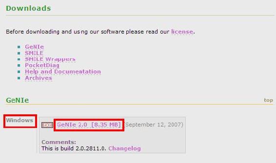
A Downloads page with several download options will appear. Click on the GeNIe 2.0 link highlighted in red on the figure below. This will initiate the download.

NOTE: The Genie Software download is only available for Windows.

Install the software by following the steps indicated in the Genie installation program.

The installation of the Genie software is now complete. Please note the help section of the software features many tutorials describing how to use a wide array of functions. However, this article will be focused on the analysis of Dynamic Bayesian Networks.

• All informational materials used to create this tutorial come from GeNIe

Using GeNIe to Analyze Dynamic Bayesian Networks

If the program was installed in the default location given in the installation wizard a shortcut to GeNIe can be found in the start menu listed under All Programs. Click on the GeNIe 2.0 Icon as seen below:

The main interface will appear as shown in the figure below:

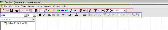
Note the important tool bars highlighted on the figure above: the menu bar (yellow), the standard toolbar (red), and the format toolbar (blue).

Consider this simple illustration of how to build a Dynamic Bayesian Network using Genie:

Polly popular is the most popular girl on the UM campus who only dates other UM students. It is common knowledge that Polly only accepts 30% of the invitations she receives to go on a date. Of the invitations that she accepts, 40% of them come from guys with high GPAs, 40% of them come from guys with medium GPAs and 20% of them come from guys with low GPAs. Of the invitations that she rejects, 10% of them come from guys with high GPAs, 30% of them come from guys with medium GPAs, and 60% of them come from guys with low GPAs.

NOTE: In this example, the variable of GPA is discretized into categories of high, medium, and low. This is necessary for analysis using Genie because otherwise there would exist infinite states for each node in the DBN (Charniak, 1991).

Creating a Bayesian network allows for determinations to be made about probabilities of Polly accepting or rejecting certain date invitations. Shown below is how to use Genie to find the probability of Polly accepting a date invitation from a guy if she knows the guy inviting her has a high GPA.

First, a node is created for the variable called acceptance of invitation. Select the “chance” node from the standard toolbar as is shown in the figure below highlighted in red.

Left-click on a clear part of the graph area of the screen. An oval will appear with “Node1” inside as seen in the figure below.

The edit mode for the node should come up automatically; if not,simply double-click on the node to pull up the edit screen as depicted in the figure below.

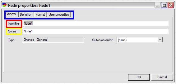
Enter an identifier for the node (must be a valid variable name in a programming language) and enter a name for the node (can be a string of any length). For this example, the identifier is entered as “Acceptance” and the name is entered as “Acceptance of Invitation”.

To define the probabilities of the node, click on the definition tab highlighted in blue as shown below. The names of the states can be edited by double clicking on the name fields (highlighted in red in the figure below) and the probabilities can be edited by clicking on the probability field (highlighted in yellow in the figure below).

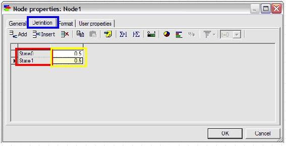
In this example, “State0” is changed to “Accept” and “State1” is changed to “Reject”. The default probabilities are entered as 0.3 for Accept and 0.7 for Reject.

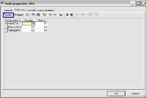
To create a second node for the variable GPA, simply click the change node again and place a second node under the “Acceptance” node. Define the name and identifier of this node as done with the “Acceptance” node. Then define the probabilities for the “GPA” node by first adding another outcome by clicking the “add outcome” button highlighted in blue in the figure below. Change state0, state1, and state2 to HighGPA, MediumGPA, and LowGPA respectively. To finish defining this node, fill in the probabilities listed in the problem statement (shown in the figure below) and press ok.

After the creation and definition of both nodes, connect these two nodes with an influence arc to represent that GPA affects how Polly accepts or rejects the invitations she receives. To do this, click on the Arc tool (found on the standard toolbar), , and click on the “Acceptance” node and drag the arrow to the new “GPA” node.

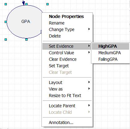
The Bayesian network describing this problem is now fully defined within the Genie program. To determine the probability of Polly accepting a date invitation from a guy if she knows the guy has a high GPA, first right click on the GPA node, scroll down to "Set Evidence", and select "HighGPA". This is shown in the figure below.

Figure below.

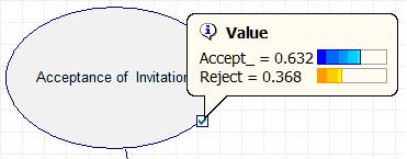
The results can also be accessed by double clicking the Acceptance node and selecting the value tab, shown in the figure below.

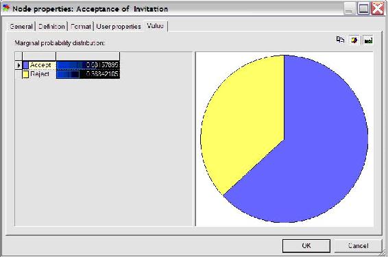
As can be seen in the figure above, Polly will accept the date invitation 63.16% of the time when she knows the guy inviting her has a high GPA. Other probabilities related to this example can be determined similarly.

The logic and procedure involved in this simple problem can be applied to complex systems with many interconnected nodes. Please see the Worked Out Examples sections for more examples of how to use Genie to analyze Bayesian networks.

• All informational materials used to create this tutorial come from GeNIe

Example \(\PageIndex{1}\)

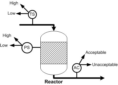
For the reactor shown below, the probability that the effluent stream will contain the acceptable mole fraction of product is 0.5. For the same reactor, if the effluent stream contains the acceptable mole fraction, the probability that the pressure of the reactor is high is 0.7. If the effluent stream does not contain the acceptable fraction, the probability that the pressure is low is 0.85. If the pressure of the reactor is high, the probability that the temperature of the feed is high is 0.9 and if the pressure of the reactor is low, the probability that temperature of the feed is low is 0.75. Given that the temperature of the feed is low, what is the probability that the effluent stream contains the acceptable mole fraction of product?

Solution

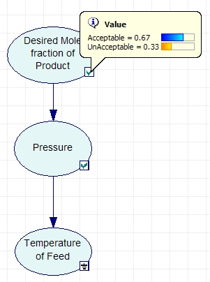
The variables to be included in the Bayesian network are the acceptable mole fraction of product in the effluent stream, the pressure of the reactor, and the temperature of the reactor. The variables are connected in an acyclic network as shown in the image below. After the nodes were created and the incidence arcs were defined, the probability was calculated by updating the network and moving the pointer over the checkmark on the node. As can be seen in the figure, the probability of the effluent stream containing the acceptable mole fraction of product given that the feed temperature is low is 67%.

A GeNIe file containing the full solution of the problem is located here. In this file, the values entered into Genie for the probabilities and stages can be accessed by double-clicking on the nodes.

Example \(\PageIndex{2}\)

The following example is complicated and contains many layers of information. It is intended to illustrate how many elements can be put together in a Bayesian Network and analyzed using Genie such that the problem is not impossibly complicated. Assume that detailed statistical experiments were conducted to find all the stated probabilities.

Consider a CSTR with a cooling jacket and an exothermic reaction with A --> B. The feed stream is pure A and the cooling stream in the jacket has a sufficient flow rate high such that the ambient temperature is constant.

The pumps transporting the reactor feed stream are old, and sometimes do not pump at their full capacity. 98% of the time the pumps work normally, but at other times the feed flow rate is slightly lower than normal. The preheating process for the feed stream is inefficient, and sometimes does not heat the reactants to 80°C. There is a 95% chance the feed stream is slightly cooler than desired. Finally, the pumps for the cooling water sometimes lose power, causing the ambient temperature for the reactor to climb higher than usual. There is a 1% chance of this power loss occurring.

The concentration of A in the reactor depends on the feed flow rate. If this flow rate is normal, then there is a 98% chance CA is normal, and a 1% chance each that it is slightly higher or lower than normal. If the flow rate is low, then there is a 40% chance that CA will be higher than normal and a 60% chance that CA will be normal.

The reactor temperature depends on the feed temperature and the ambient temperature. If both T0 and Ta are normal, there is a 98% chance T is normal, and a 1% chance each that it is slightly higher or lower than normal. If T0 is normal and Ta is high, there is a 90% chance T is normal and a 10% chance it is high. If Ta is normal and T0 is low, there is a 80% chance T is normal and a 20% T is low. Finally, if T0 is low and Ta is high, there is a 90% chance T is normal, a 8% chance T is low, and a 2% chance T is high.

The conversion depends on CA and T. If one of these variables is high and the other low, there is an equal chance that X will be low, normal, or high. If both CA and T are normal, there is a 98% chance X is normal, and a 1% chance each that it is slightly higher or lower than normal. If both CA and T are low, there is equal chance that X will be low or normal. If both CA and T are high, there is equal chance that X will be normal or high. If CA is normal and T is low, there is a 75% chance X is normal and a 25% chance X is low. If CA is normal and T is high, there is a 75% chance X is normal and a 25% chance X is high. Finally, if T is normal and CA is low or high, there is a 85% chance X is normal and a 15% chance that X is low or high, respectively.

Create a model in Genie for this system that can be used to determine probabilities of related events occuring.

Solution

A GeNIe file containing the Bayesian Network of this problem is located here.

This model can be used to answer questions such as (1) if a composition sensor for B in the exit stream tells us that the conversion is slightly low, what is the probability that the feed temperature is normal and (2) if a temperature sensor in the reactor tells us that the reactor temperature is high what is the probability that the ambient temperature is normal?

miniTuba

MiniTuba is a program that allows the creation of Bayesain Networks thought time, with only the final data sets. This was created by Zuoshuang Xiang, Rebecca M. Minter, Xiaoming Bi, Peter Woolf, and Yongqun He, to analysis medical data, but can be used to create Bayesian Networks for any propose. In oder to use this program go to www.minituba.org/ and go to the Sandbox demo Tab. From here one can either start a new project or merly modify an old project. This wiki will talk though how to create a new project.

First Log in: to do this click the Log In link at the bottom of the page and enter demo@e.d.u as the user name and demo as the password this should bring up this screen:

and click My Projects and then Creat New Project.

The user needs to know how many variables (EX: Temperature, Pump speed, Yield, flowrate in ChemE), data sets (EX: Reactors, Tanks etc.) and the average number of time steps that will be analyzed.

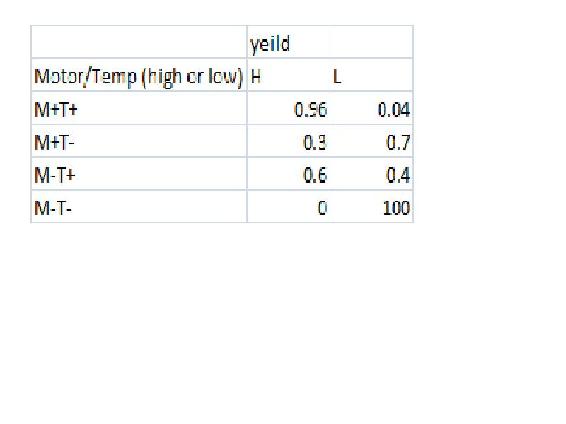
In this example we will have a CSTR whose yield may be affected by the reactor Volume, the motor speed, the temperature or the concentration. This means that there are 5 variable. Lets say that we have 5 reactors running this experiment with differing either high or low Moter speed, temperature, and yield and either high medium or low volume and concentration. In this example Yield is only affected by the motor speed and Temperature with the following probability

Enter the requested data in miniTuba and then click open project from the list. Then click "load/updata data"

this example will use the following data:

Media:CSTRExample.xls

To insert the data, simply copy and paste in the data to open box, then click LOAD DATA. In Order to run the analysis click "Start DBN botton"

Here you can slect which data series and variables you would like to analize. Now miniTuba gives several different options for the data. The data can be analyises and a child a parent or both. A Child means that the data isnt effected by the other datathat , Parent means the data doesnt affect the other data, and both means that the data can be affected and effect other variables. In our example, the motor speed is the only thing that we know is not affected by teh other variables, so we will select it as a parent.

Discretization Policy tells MiniTuba how to bin the. In our case, as things are exactly high, med or low represented by 0,1,2 it is easy to desice how to descretize the data, but it is ok if the data isnt allready bin (ie in 0s 1s and 2s). Quantile spits the data into even chucks (ie if you select quantile 2, it will find the mean and then everything above that is in one bin and everything below that mean is in a different bin). Interval bins things that are in equal sized intervals around each other.

Select Natural fit for slipe fitting (this will allow you to have some data points missing ex: no volume reading in 1 data set) Lets select 2 intervals for moter speed, temperature and yeild adn then 3 intervals for volume and concentration.

MiniTuba also give you the option to force it to come up with some relationships weather MiniTuba thinks they should or not. MiniTuba also allows you to choose the method used to solve this, we will select simulated anneling Number of Instances allows you to choose the number of computers used to solve the problem, we will just leave it at 1 In the Demo version, the max calculation time is 1 min.

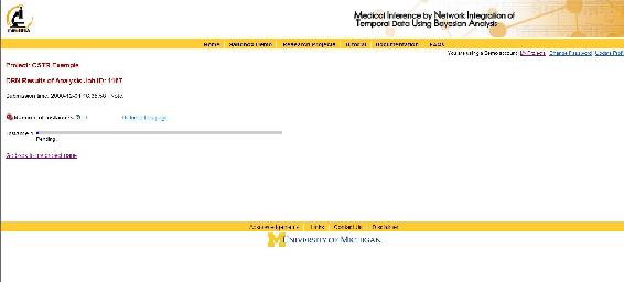
When everything is done, click Run Bayesian Analysis. By clicking Check Progress teh following screen will show up. Click Updata every so often to check weather the solution has been computed.

This will output the following screen when it is done

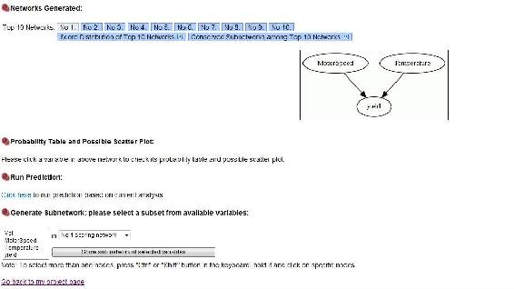
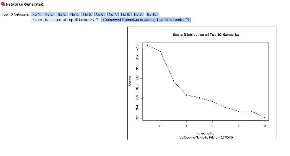
As you can see, the yield depends on the motor speed and the temperature alone, just like we crated the module to show. Top Ten networks, shows the 10 most likely networks. Click Score Distribution of Top Ten Networks shows the relative probability of each network, and the probability that the number 1 network is the correct network out of the top 10. In our example the best network has a probablitity of 0.77 as seen below.

References

• Charniak, Eugene (1991). "Bayesian Networks without Tears", AI Magazine, 50-62.
• GeNIe Helpfile at GeNIe & SMILE
• Murphy, Kevin. (2002). "Dynamic Bayesian Networks."
• Xiang Z., Minter R., Bi X., Woolf P., and He Y.(2007). "miniTUBA: medical inference by network integration of temporal data using Bayesian analysis," Bioinformatics, v. 23, 2423-2432, 2007.

Contributors and Attributions

• Authors: Kevin Dahlberg, Paul Jantzen, Genevieve Lampinen, Albert Sawalha, and David Toronto
• Stewards: Ross Bredeweg, Jessica Morga, Ryan Sekol, Ryan Wong