13.7: Occasionally Dishonest Casino? Markov Chains and Hidden Markov Models

Last updated
Save as PDF

Page ID: 22528

$ \newcommand{\vecs}[1]{\overset { \scriptstyle \rightharpoonup} {\mathbf{#1}} } $ $ \newcommand{\vecd}[1]{\overset{-\!-\!\rightharpoonup}{\vphantom{a}\smash {#1}}} $$\newcommand{\id}{\mathrm{id}}$ $ \newcommand{\Span}{\mathrm{span}}$ $ \newcommand{\kernel}{\mathrm{null}\,}$ $ \newcommand{\range}{\mathrm{range}\,}$ $ \newcommand{\RealPart}{\mathrm{Re}}$ $ \newcommand{\ImaginaryPart}{\mathrm{Im}}$ $ \newcommand{\Argument}{\mathrm{Arg}}$ $ \newcommand{\norm}[1]{\| #1 \|}$ $ \newcommand{\inner}[2]{\langle #1, #2 \rangle}$ $ \newcommand{\Span}{\mathrm{span}}$ $\newcommand{\id}{\mathrm{id}}$ $ \newcommand{\Span}{\mathrm{span}}$ $ \newcommand{\kernel}{\mathrm{null}\,}$ $ \newcommand{\range}{\mathrm{range}\,}$ $ \newcommand{\RealPart}{\mathrm{Re}}$ $ \newcommand{\ImaginaryPart}{\mathrm{Im}}$ $ \newcommand{\Argument}{\mathrm{Arg}}$ $ \newcommand{\norm}[1]{\| #1 \|}$ $ \newcommand{\inner}[2]{\langle #1, #2 \rangle}$ $ \newcommand{\Span}{\mathrm{span}}$$\newcommand{\AA}{\unicode[.8,0]{x212B}}$

Introduction

Basic probability can be used to predict simple events, such as the likelihood a tossed coin will land on heads rather than tails. Instinctively, we could say that there is a 50% chance that the coin will land on heads.

But let’s say that we’ve just watched the same coin land on heads five times in a row, would we still say that there is a 50% chance of the sixth coin toss will results in heads? No – intuitively, we sense that there is a very low probability (much less than 50%) that the coin will land on heads six times in a row.

What causes us to rethink the probability of the coin landing on heads? The same coin is being tossed, but now we are taking into account the results of previous tosses. Basic probability can be used to predict an isolated event. But more advanced probability concepts must be used to assess the likelihood of a certain sequence of events occurring. This section provides an introduction to concepts such as Bayes rule, Markov chains, and hidden Markov models, which are more useful for predicting real world scenarios (which are rarely singular, isolated events).

Bayes' Rule

Bayes’ rule is a foundational concept for finding the probability of related series of events. It relates the probability of event A conditional to event B and the probability of event B conditional to event A, which are often not the same probabilities.

\[P(A | B)=\frac{P(B | A) P(A)}{P(B)} \nonumber \]

Another interpretation of Bayes’ rule: it’s a method for updating or revising beliefs (i.e. probability of landing on heads) in light of new evidence (knowing that the coin landed on heads the last five tosses).

Markov Chains

A Markov chain is a particular way of modeling the probability of a series of events. A Markov chain is a sequence of random values whose probabilities at a time interval depend only upon the value of the number at the previous time. A Markov chain, named after Andrey Markov, is a stochastic process with the Markov property. This means that, given the present state, future states are independent of the past states. In other words, the description of the present state fully captures all the information that could influence the future evolution of the process, so that future states of the system will be reached through a probabilistic (determined from current data) process instead of a deterministic one (from past data).

At each point in time, the system could either change its state from the current state to a different state, or remain in the same state. This happens in accordance with the specified probability distribution. These changes of state are called transitions, and the probabilities associated with various state changes are called transition probabilities.

For example, let’s say we want to know the probability of an elevator moving more than five floors up in a 30-floor building (including the lobby). This is an example of a Markov chain because the probability does not depend on whether the elevator was on the 6th floor at 7:00 am or on the 27th floor at 10:30 pm. Instead the probability is dependent on what floor the elevator is on right before it starts to move. More specifically, the fact that the elevator is on the top floor at $t_1$ results in a zero probability that the elevator will be five floors higher at $t_2$.

The figure below helps to visualize the concept of a Markov Model.

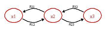
x₁, x₂, x₃ = states

a₁₂, a₂₁, a₂₃, a₃₂ = transition probabilities

A transition probability is simply the probability of going from one state to another state. Please note that there may be other paths or transition probabilities for state x₁, say to state x₃ or back to itself. The sum of the transition probabilities must always equal to 1.

\[a_{1, i}=a_{11}+a_{12}+a_{13}+\ldots a_{1 n} \nonumber \]

\[\sum_i=1 \nonumber \]

Transition Probability

The transition probabilities of each state for one system can be compiled into a transition matrix. The transition matrix for a system can represent a one-step transition or a multiple-step transition. A n-step transition matrix is simply a one-step transition matrix raised to the n-th power.

For state i to make a transition into state j, the transition probability P_ij must be greater than 0. so:

\[P_{i, j} \geq 0, i, j \geq 0 \nonumber \]

\[\sum_{j=0} P_{ij} = 1 \nonumber \]

with $i$ = 0, 1, ...

Let P be the matrix of a one-step transition matrix,

P=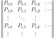 $begin{Vmatrix} P_{0,0} & P_{0,1} & P_{0,2} & \cdots \\ P_{1,0} & P_{1,1} & P_{1,2} & \cdots \\ \vdots & \ddots & \vdots \\ P_{i,0} & P_{i,1} & P_{i,2} & \cdots \\ \vdots & \vdots & \vdots \end{Vmatrix}$

$P_{i,1}$ would denote the probability of going from state i to 1

Example $\PageIndex{1}$: Will It Rain Tomorrow?

Suppose that whether or not it rains today depends on previous weather conditions through the last two days. Specifically, suppose that if it has rained for the past two days, then it will rain tomorrow with probability 0.7; if it rained today but not yesterday, then it will rain tomorrow with probability 0.5; if it rained yesterday but not today, then it will rain tomorrow with probability 0.4; if it has not rained in the past two days, then it will rain tomorrow with probability 0.2.

Solution

The transition matrix for the above system would be:

state 0: if it rained both today and yesterday
state 1: if it rained today but not yesterday
state 2: if it rained yesterday but not today
state 3: if it did not rain either yesterday or today

\[\mathbf{P}=\left| \begin{array}{cccc}
0.7 & 0 & 0.3 & 0 \\
0.5 & 0 & 0.5 & 0 \\
0 & 0.4 & 0 & 0.6 \\
0 & 0.2 & 0 & 0.8 \right|
\end{array} \nonumber \]

Applications of Markov Chains

Since this concept is quite theoretical, examples of applications of this theory are necessary to explain the power this theory has. Although these following applications are not chemical control related, they have merit in explaining the diversity of operations in which Markov chains can be used. Hopefully, by seeing these examples, the reader will be able to use Markov chains in new, creative approaches to solve chemical controls problems.

Queuing Theory

Markov chains can be applied to model various elements in something called queuing theory. Queuing theory is simply the mathematical study of waiting lines (or queues).

This theory allows for the analysis of elements arriving at the back of the line, waiting in the line, and being processed (or served) at the front of the line. This method uses the variables including the average waiting time in the queue or the system, the expected number waiting or receiving service and the probability of encountering the system in certain states, such as empty, full, having an available server or having to wait a certain time to be served. These variables are all unique to the system at hand. A link that explains this theory in more detail can be found below:

Queueing Theory

Although Queuing Theory is generally used in customer service, logistics and operations applications, it can be tailored to chemical processing. For instance, it is essential to model how long a particular product will be in an assembly line before it makes it to the desired end process. Thus, this theory is robust for all kinds of uses.

Example $\PageIndex{1}$: Queuing Problem

On a sunny Tuesday morning in the Computer Engineering Building, a group of Chemical Engineering students are finishing their engineering laboratory reports and have stayed up all night writing ambivalent fluid mechanics questions, they need some prestigious coffee for refreshment instead of Red Bull. Coffee shop called "Dreamcaster's Cafè" was opened by a University of Michigan Chemical Engineering graduate. Business is going very well for "Dreamcaster's Cafè" and there are many people, m people, waiting in line in front of the Chemical Engineering students. The service time for the first person in line (not necessarily a Chemical Engineering student) is an exponential distribution with an average waiting time of $\frac{1}{\mu}$ . Since the Chemical Engineering students have to return to the Computer Engineering Building to finish their report, they have a finite patience waiting in line and their patience is an exponential distribution with an average of $\frac{1}{\theta}$ . The group of Chemical Engineering students does not care how long the service time is. Find the probability that the ith Chemical Engineering student to wait long enough to get coffee.

Solution

ueuing Problem.jpg

Add text here.

Google’s Page Ranking System

The PageRank of a webpage as used by Google is defined by a Markov chain. PageRank is the probability to be at page $i$ in the following Markov chain on all (known) webpages. If N is the number of known webpages, and a page $i$ has $k_i$ links then it has transition probability

\[\dfrac{(1 − q)}{ki} + \dfrac{q}{N} \nonumber \]

for all pages that are linked to and $q/N$ for all pages that are not linked. The constant $q$ is around 0.15.

Children’s Games

Markov chains are used in the children’s games “Chutes and Ladders,” “Candy Land” and “Hi Ho! Cherry-O!” These games utilize the Markov concept that each player starts in a given position on the game board at the beginning of each turn. From there, the player has fixed odds of moving to other positions.

To go into further detail, any version of Snakes and Ladders can be represented exactly as a Markov chain, since from any square the odds of moving to any other square are fixed and independent of any previous game history. The Milton Bradley version of Chutes and Ladders has 100 squares, with 19 chutes and ladders. A player will need an average of 45.6 spins to move from the starting point, which is off the board, to square 100.

I Prob.gif

One last game of interest is Monopoly. This can be modeled using Markov chains. Check out the following link to see a simulation of the probability of landing on a particular property in the Monopoly game:

Monopoly Simulation

Hidden Markov Models

Building further on the concept of a Markov chain is the hidden Markov model (HMM). A hidden Markov model is a statistical model where the system being modeled is assumed to be a Markov process with unknown parameters or casual events. HMMs are primarily helpful in determining the hidden parameters from the observable parameters.

Again, the figure below may help visualize the Hidden Markov Model concept.

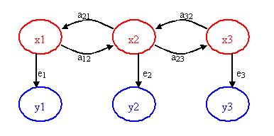
x₁, x₂, x₃ = hidden/unknown states

a₁₂, a₂₁, a₂₃, a₃₂ = transition probabilities

y₁, y₂, y₃ = observable states

e₁, e₂, e₃ = emission probabilities

The key point of the figure above is that only the blue circles are seen, but you suspect or know that these observable states are directly related or dependent on some hidden state. These hidden states (the red circles) are what actually dictates the outcome of the observable states. The challenge is to figure out the hidden states, the emission probabilities and transition probabilities.

For example, say you have a data acquisition program that continuously records the outlet temperature of your product stream which you are heating up through a heat exchanger. The heat exchanger provides a constant supply of heat. You observe that the temperature has some step disturbances and is not always constant. The temperature is the observable parameter, but the cause of its deviations/states is actually the stream's flowrate. When the flowrate fluctuates, the outlet temperature also fluctuates since the heat exchanger is providing the same amount of heat to the stream. So, the stream flowrate is the hidden parameter (since you do not have access to this measured variable) and the probability that the flowrates switches from say 100 to 150 to 300 L/h are the transition probabilities. The emission probability is the probability that the observed outlet temperature is directly caused by the flowrate. This emission probability is not necessarily 1 since temperature variations could also be due to noise, etc.

Another common scenario used to teach the concept of a hidden Markov model is the “Occasionally Dishonest Casino”. If a casino uses a fair die, each number has a 1/6 probability of being landed on. This type of probability that represents a known parameter is known as emission probability in HMMs. Sometimes a casino can tip the odds by using a loaded die, where one number is favored over the other five numbers and therefore the side that is favored has a probability that is higher than 1/6.

But how does one know that the casino is being dishonest by using a loaded die? Pretend that the die is loaded in such a way that it favors the number 6. It would be difficult to differentiate between a fair die and loaded die after watching only one roll. You may be able to get a better idea after watching a few tosses and see how many times the die landed on 6. Let’s say that you saw the following sequence of die tosses:

465136

It is still difficult to say with certainty whether the die is loaded or not. The above sequence is a feasible for both a fair die and a loaded die. In this particular case, the above numbers that represent what was rolled are the observable parameters. The hidden parameter is the type of die used just because we do not know which type produced the above sequence of numbers.

Instead of relying on a sneaking suspicion that the casino is being dishonest, one can use a hidden Markov model to prove that a loaded die is being used occasionally. Please note that if a loaded die was used all the time it would be more blatantly obvious. In order to get away with this “slight” unfairness, the casino will switch the fair die with a loaded one every so often. Let’s say that if a fair die is being used there is a 5% chance that it will be switched to a loaded die and a 95% chance that it will remain fair. These are known as transition probabilities because they represent the likelihood of a causal event changing to another causal event.

Below is a picture representing the transition probabilities (probability of staying or changing a type of die) as well as the emission probabilities (probability of landing on a number).

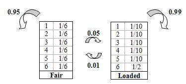
Using the basic diagram above that show the emission and transition properties, conditioned statements in Excel can be used to model the probability that a loaded die is being used. Please refer to example two for the hidden Markov model Excel sheet.

HHMs can be modeled using Matlab. Follow the link to the site which contains information in installing the HHM toolbox in Matlab:

HHMs in Matlab

Example $\PageIndex{1}$: "What should I wear?"

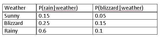
The weather affects important issues such as, choice of clothing, shoes, washing your hair, and so many more. Considering the bizarre weather in Ann Arbor, you wish to be able to calculate the probability that it will rain given the data of the last three consecutive days. Applying your chemical engineering skills and empowered by the knowledge from this Wiki article, you sit down and decide to be the next Weather-Person.

You know the following information since you have been an avid fan of the Weather Channel since age 5.

eatherTable 1updated.JPG

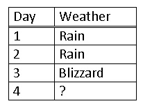
You then record the weather for the past 3 days.

Solution

Since the last day was a blizzard you use a matrix expressing a 100% chance in the past, and multiply this by the probabilities of each weather type.

\[\left[\begin{array}{lll}
0 & 1 & 1
\end{array}\right]\left[\begin{array}{ccc}
8 & 15 & 05 \\
.6 & 25 & .15 \\
3 & .6 & .1
\end{array}\right]=\left[\begin{array}{lll}
.6 & .25 & .15
\end{array}\right] \nonumber \]

This means that there is a 60% chance of sun, a 25% chance of rain and a 15% chance of a blizzard. This is because a Markov process works based on the probability of the immediately previous event. Thus, you decide that is a low enough risk and happily decide to wear your best new outfit AND wash your hair.

Example $\PageIndex{2}$: "What should I wear for the weekend?"

Turns out it does rain the next day and you get your favorite clothes soaked. However, you are leaving for a weekend with your family and must decide what to wear for the next two days. What is the prediction for the next two days?

Solution

Predicting for the first day is like the previous example substituting rain in for a blizzard.

\[\left[\begin{array}{lll}
0 & 0 & 1
\end{array}\right]\left[\begin{array}{ccc}
.8 & .15 & .05 \\
.6 & .25 & .15 \\
.3 & .6 & .1
\end{array}\right]=\left[\begin{array}{lll}
.3 & .6 & .1
\end{array}\right] \nonumber \]

In order to predict for the second day we must use our previous data to predict how the weather will act. Since we predict two days ahead we multiply the probabilities twice, effectively squaring them.

\[\left[\begin{array}{lll}
0 & 0 & 1
\end{array}\right]\left[\begin{array}{lll}
8 & 15 & 05 \\
6 & 25 & .15 \\
3 & 6 & .1
\end{array}\right]^{2}=\left[\begin{array}{llll}
.63 & .255 & .115
\end{array}\right] \nonumber \]

Alternatively, we can take the prediction from the previous day and multiply that by the probability of weather.

\[\begin{array}{lllll}
\text { L. } 3 & .6 & 1\rfloor & .0 & .15 & .05 \\
.6 & .25 & .15 & =.63 & .255 & .115
\end{array} \nonumber \]

Both ways give you the same answer. Therefore, you decide to pack for both sunny and rainy weather.

Example $\PageIndex{3}$: OSEH Example

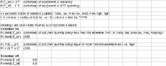
Now, back to REAL chemical engineering applications, the probability theories described above can be used to check if a piece of equipment is working. For example, you are an OSEH inspector and you have to analyze a set of data recording the pollutant levels of a plant. If they use the scrubber they have, the probability of pollutant levels being high is low. However, if the scrubber is not used, the probability of pollutant levels being high increases. You have gotten some inside information that the operators use the scrubbers only 70% off the time. Your task is to create a model based on the data recordings and using probability theories to predict WHEN they switch their scrubbers ON and OFF, so that you can catch them red-handed in the act!

There are 6 possible pollutant levels: none, low, med-low, med, med-high, and high. If the level = high, then this is above the allowable limit. Every other level is considered allowable. If the scrubber is ON, there is equal chance that any of the states will occur. If the scrubber is OFF, there is a 50% chance that a high pollutant level will be recorded.

Given the following data:

Solution

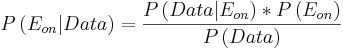
Formulas used are listed below:

(1) $\left( Data|E_{on} \right)=P \left(<limit|E_{on} \right)^{n-1}P\left(limit|E_{on} \right)^{n}= \left(\frac{5}{6}\right)^{n-1}\left(\frac{1}{6}\right)^{n}$

(2) $\left( Data|E_{off} \right)=P \left(<limit|E_{off} \right)^{n-1}P\left(limit|E_{off} \right)^{n}=\left(\frac{1}{2}\right)^{n-1}\left(\frac{1}{2}\right)^{n}$

(3) $\left( Data \right)=P \left(Data|E_{on} \right)*P\left(E_{on}\right)+P\left(Data|E_{off} \right)*P\left(E_{off}\right)$

(4) $\left( E_{on}|Data \right)=\frac{P \left(Data|E_{on} \right)*P\left(E_{on}\right)}{P\left(Data \right)}$

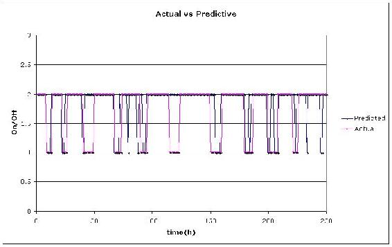
Please refer to the attached Excel File for the predictive model. OSEHExample

From our results in the Excel file, we graphed the predicted vs actual times when the scrubber was turned off. The value of "1" was chosen arbitrarily to represent when the scrubber was OFF and "2" when it was "ON".

Multiple Choice Question 1

What is the key property of a Markov chain?

A) Probability of each symbol depends on FUTURE symbols.

B) Probability of each symbol depends on ALL preceding symbols.

C) Probability of each symbol depends on NONE of the preceding symbols.

D) Probability of each symbol depends only on the value of the PREVIOUS symbol.

Multiple Choice Question 2

What kind of parameters does emission probability represent?

A) unknown parameters

B) Markov parameters

C) known parameters

D) Bayes' parameters

References

Woolf P., Keating A., Burge C., and Michael Y. "Statistics and Probability Primer for Computational Biologists". Massachusetts Institute of Technology, BE 490/ Bio7.91, Spring 2004
Smith W. and Gonic L. "Cartoon Guide to Statistics". Harper Perennial, 1993.
Kemeny J., Snell J. "Finite Markov Chains". Springer, 1976. ISBN 0387901922
en.Wikipedia.org/wiki/Snakes_and_Ladders
Page, Lawrence; Brin, Sergey; Motwani, Rajeev and Winograd, Terry (1999). "The PageRank citation ranking: Bringing order to the Web"

Use the Harvard Referencing style for references in the document.
For more information on when to reference see the following Wikipedia entry.
Ross, Sheldon M. "Introduction to Probability Models". Academic Press, 2007.

Contributors

Authors: Nicole Blan, Jessica Nunn, Pamela Roxas, Cynthia Sequerah
Stewards: Kyle Goszyk, So Hyun Ahn, Sam Seo, Mike Peters

Search

Example \(\PageIndex{1}\): Will It Rain Tomorrow?

Solution

Example \(\PageIndex{1}\): Queuing Problem

Solution

Example \(\PageIndex{1}\): "What should I wear?"

Solution

Example \(\PageIndex{2}\): "What should I wear for the weekend?"

Solution

Example \(\PageIndex{3}\): OSEH Example

Solution