17.5: Obtaining Stability and Performance- A Preview

In the lectures ahead we will be concerned with developing analysis and synthesis tools for studying stability and performance in the presence of plant uncertainty and system disturbances.

Stabilization

Stabilization is the first requirement in control design - without stability, one has nothing! There are two relevant notions of stability:

(a) nominal stability (stability in the absence of modeling errors), and

(b) robust stability (stability in the presence of some modeling errors).

In the previous sections, we have shown that stability analysis of an interconnected feedback system requires checking the stability of the closed-loop operator, \(\mathcal{T}(P, K)\). In the case where

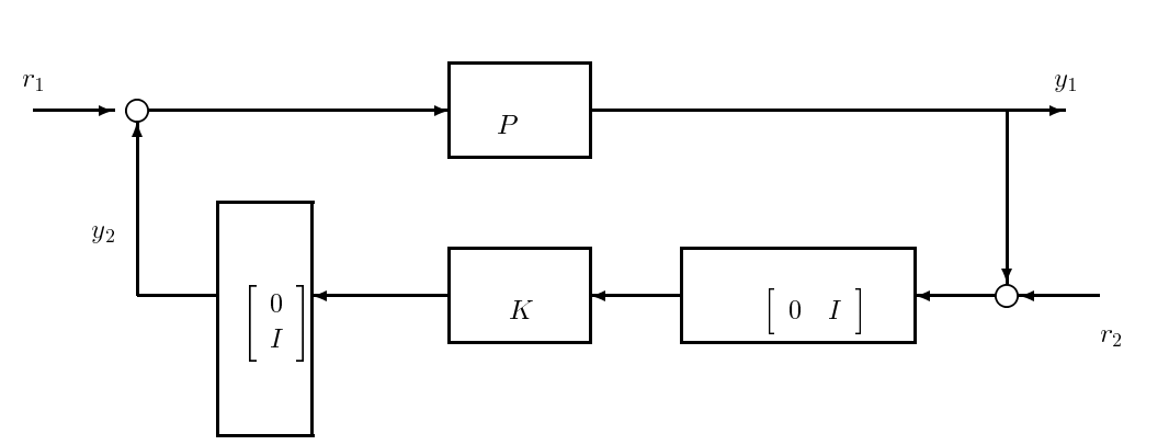
Figure \(\PageIndex{1}\): A more general feedback configuration.

modeling errors are present, such a check has to be done for every possible perturbation of the system. Efficient methods for performing this check for specified classes of modeling errors are necessary.

Meeting Performance Specifications

Performance specifications (once stability has been ensured) include disturbance rejection, command following (i.e., tracking), and noise rejection. Again, we consider two notions of performance:

(a) nominal performance (performance in the absence of modeling errors), and

(b) robust performance (performance in the presence of modeling errors).

Many of the performance specifications that one may want to impose on a feedback system can be classified under the following two types of specifications:

1. Disturbance Rejection This corresponds to minimizing the effect of the exogenous inputs \(w\) on the regulated variables \(z\) in the general 2-input 2-output description, when the exogenous inputs are only partially known. To address this problem, it is necessary to provide a model for the exogenous variables. One possibility is to assume that \(w\) has finite energy but is otherwise unknown. If we desire to minimize the energy in the \(z\) produced by this \(w\), we can pose the performance task as involving the minimization of

\[\sup _{w \neq 0} \frac{\|\Phi w\|_{2}}{\|w\|_{2}}\nonumber\]

where \(\Phi\) is the map relating \(w\) to \(z\). This is just the square root of the energy-energy gain, and is measured by the \(\mathcal{H}_{\infty}\)-norm of \(\Phi\).

Alternatively, if \(w\) is assumed to have finite peak magnitude, and we are interested in the peak magnitude of the regulated output \(z\), then the measure of performance is given by the peak-peak gain of the system, which is measured by the `\(l_{1} / \mathcal{L}_{1}\)-norm of \(\Phi\). Other alternatives such as power-power amplification can be considered.

A rather different approach, and one that is quite powerful in the linear setting, is to model \(w\) as a stochastic process (e.g, white noise process). By measuring the variance of \(z\), we obtain a peformance measure on \(\Phi\).

2. Fixed-Input Specifications. These specifications are based on a specific command or nominal trajectory. One can, for instance, specify a template in the time-domain within which the output is required to remain for a given class of inputs. Familiar specifications such as overshoot, undershoot, and settling time for a step input fall in this category.

Finally, conditions for checking whether a system meets a given performance measure in the presence of prescribed modeling errors have to be developed. These topics will be revisited later on in this course.