18.1: SISO Loop Shaping

The Classical Viewpoint

The standard "servo" or tracking configuration of classical feedback control is shown in Figure 18.1. In this arrangement, the controller \(K\) is fed by an error signal \(e\), which is the difference between a reference \(r\) and the measured output \(y\) of the plant \(P\). The measurement is perhaps corrupted by noise \(n\). The output of the controller is the input \(u\) to the plant. In addition, external disturbances may drive the plant, and are represented here via the signal \(d\) added in at the output of the plant. In a typical classical control design, the compensator \(K\) would be picked as the lowest-order system that ensures the following:

1. the closed-loop system is stable;

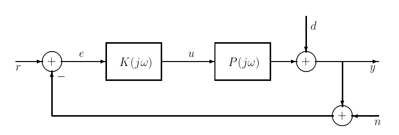
Figure \(\PageIndex{1}\): Standard feedback configuration with noise, disturbance, and reference inputs.

2. the loop gain \(P(j \omega) K(j \omega)\) has large magnitude at frequencies (low frequencies, typically) where the power of the plant disturbance \(d\) or reference input \(r\) is concentrated.

3. the loop gain has small magnitude at frequencies (high frequencies, typically) where the power of the measurement noise \(n\) is concentrated.

The need for the first requirement is clear. The origins of the second and third requirements will be explained below. In order to simultaneously attain all three objectives, it is most convenient to have a criterion for closed-loop stability that is stated in terms of the (openloop) loop gain, and this is provided by the Nyquist stability criterion.

The reasons for the second and third requirements above lie in the sensitivities of the closed-loop system to plant disturbances, reference signals, and measurement noise. Let \(S\) denote the transfer function that maps a disturbance \(d\) to the output \(y\) in the closed-loop system. This \(S\) is termed the (output) sensitivity function, and for the arrangement in Figure 18.1 it is given by

\[S=(1+P K)^{-1} \ \tag{18.1}\]

Speaking informally for the moment, if \(|P(j \omega) K(j \omega)|\) is large at frequencies where (in some sense) the power of \(d\) is concentrated, then \(|S(j \omega)|\) will be small there, so the effect of the disturbance on the output will be attenuated. Since plant disturbances are typically concentrated around the low end of the frequency spectrum, one would want \(|P(j \omega) K(j \omega)|\) to be large at low frequencies. Thus, disturbance rejection is a key motivation behind classical control's low-frequency specification on the loop gain.

Note that (in the SISO case) \(S\) is also the transfer function from \(r\) to \(e\). If we want \(y\) to track \(r\) with good accuracy, then we want a small response of the error signal \(e\) to the driving signal \(r\). This again leads us to ask for \(|S(j \omega)|\) to be small - or equivalently for \(|P(j \omega) K(j \omega)|\) to be large - at frequencies where the power of the reference signal \(r\) is concentrated. Fortunately, in many (if not most) control applications, the reference signal is slowly varying, so this requirement again reduces to asking for \(|P(j \omega) K(j \omega)|\) to be large at low frequencies. Thus, tracking accuracy is another motivation behind classical control's low-frequency specification on the loop gain.

In contrast, the motivation behind classical control's high frequency specification is noise rejection. Let \(T\) denote the transfer function that maps the noise input \(n\) to the output \(y\). Given the arrangement in Figure 18.1,

\[T=P K(1+P K)^{-1} \ \tag{18.2}\]

This \(T\) is termed the complementary sensitivity function, because

\( T + S = 1 \ \tag{18.3}\]

Note that \(T\) is also the transfer function from \(r\) to \(y\). If \(|P(j \omega) K(j \omega)|\) is small at frequencies where the power in \(n\) is concentrated, then \(|T(j \omega)|\) will be small there, so the effect of the noise on the output will be attenuated. Measurement noise tends to occur at higher frequencies, so to minimize its effects on the output, we typically specify that \(|P(j \omega) K(j \omega)|\) be small at high frequencies. This constraint fortunately does not conflict with the low-frequency constraints imposed above by typical \(d\) and \(r\). Also, the constraint is well matched to the inevitable fact that the gain of physical systems will eventually fall off with frequency.

The picture of the control design task that emerges from the above discussion is the following: Given the plant \(P\), one typically needs to pick the compensator \(K\) so as to obtain a loop gain magnitude \(|P(j \omega) K(j \omega)|\) that is large at low frequencies, "rolls off" to low values at high frequencies, and varies in such a way that the Nyquist stability criterion is satisfied. [For the special case of open-loop stable plants and compensators, the stability condition can be stated in alternative forms that are easy to check using Bode plots rather than Nyquist plots, and this can be more convenient. The standard rule of thumb focuses on the roll-off around the crossover frequency \(\omega_{c}\), defined as the frequency where the loop gain magnitude is unity; this frequency is a crude measure of closed-loop bandwidth. The specification is that the roll-off of the loop gain magnitude around \(\omega_{c}\) should be no steeper than -20dB/decade. Furthermore, \(\omega_{c}\) should be picked below frequencies where the loop gain is significantly affected by any right-half-plane zeros of the loop transfer function \(P K\); this provides an initial indication that right-half-plane zeros can limit the attainable closed-loop performance.]

A Modern Viewpoint

The challenge now is to translate the above classical control design approach into something more precise and systematic, and more likely to have a natural MIMO extension. The following example points the way, and makes free use of the signal and system norms that we defined in Lectures 11 and 12.

Example 18.1 (SISO Disturbance Rejection and Weighted Sensitivity)

We have already seen that the expression relating \(y\) to \(d\) in the SISO feedback configuration depicted in Figure 18.1 is

\[y=(1+P K)^{-1} d \ \tag{18.4}\]

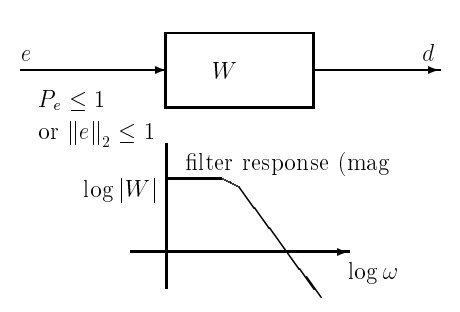
Figure \(\PageIndex{2}\): Representing the plant disturbance \(d\) as the output of a shaping filter \(W\) whose input \(e\) is an arbitrary bounded energy or bounded power signal, or possibly white noise.

Typically, \(d\) has frequency content concentrated in the low-frequency range. In order to get the requisite frequency characteristic, one might model \(d\) as the output of a shaping filter with transfer function \(W\), as shown in Figure 18.2, with the input \(e\) of the filter being an arbitrary bounded energy or bounded power disturbance (or, in the stochastic setting, white noise). Thus \(e\) has no spectral "coloring", and all the coloring of \(d\) is embodied in the frequency response of \(W\).

For the rest of this example, let us focus on the bounded energy or bounded power models for \(e\). Suppose our goal now is to choose \(K\) to minimize the effect of the disturbance \(d\) on the output \(y\). From Lectures 11 and 12, and given our model for \(d\), we know that this is equivalent to minimizing the \(\mathcal{H}_{\infty}\)-gain of the transfer function from \(e\) to \(y\), because in the case of a bounded power \(e\) this gain is the attainable or "tight" bound on the ratio of rms values at the output and input,

\[\frac{\rho_{y}}{\rho_{e}} \leq\left\|(1+P(j \omega) K(j \omega))^{-1} W(j \omega)\right\|_{\infty}\nonumber\]

while in the case of a bounded energy \(e\) we again have the tight bound

\[\frac{\|y\|_{2}}{\|e\|_{2}} \leq\left\|(1+P(j \omega) K(j \omega))^{-1} W(j \omega)\right\|_{\infty}\nonumber\]

In terms of the sensitivity function,

\[S(j \omega)=(1+P(j \omega) K(j \omega))^{-1}\nonumber\]

the task is to pick \(K\) to minimize the \(\mathcal{H}_{\infty}\) norm \(\|S(j \omega) W(j \omega)\|_{\infty}\).

If

\[\|S(j \omega) W(j \omega)\|_{\infty} \leq \gamma \ \tag{18.5}\]

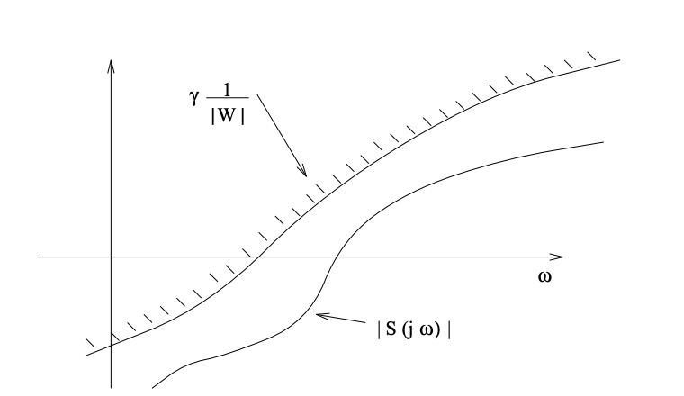
Figure \(\PageIndex{3}\): Graphical interpretation of the sensitivity function being bounded by a scaled reciprocal of the weighting filter frequency response.

then

\[|S(j \omega)||W(j \omega)| \leq \gamma, \forall \omega \ \tag{18.6}\]

This implies that

\[|S(j \omega)| \leq \gamma \frac{1}{|W(j \omega)|} \ \tag{18.7}\]

which tells us that the sensitivity function is bounded by a scaled reciprocal of the weighting filter. A graphical representation of this bound is shown in Figure 18.3. From Figure 18.3 we can see that the value \(\gamma\) and the filter \(W(j \omega)\) give us a clear picture of the constraint on the sensitivity function. This allows one to more systematically design a controller, since we directly get the closed loop characteristics. Note also that with the \(Q\)-parametrization of \(K\), the sensitivity function \(S\) is affine in \(Q\), and this form is much easier to work with than the fractional form that \(S\) takes as a function of \(K\).

The major benefit of the formulation in the above example is that a MIMO version of it is quite immediate, as we see in the next section.