20.7: Stability Robustness Analysis

Next, we present a few examples to illustrate the use of the small-gain theorem in stability robustness analysis.

Example 20.1 (Additive Perturbation)

For the configuration in Figure 20.1, it is easily seen that

\[M=-K\left(I+P_{0} K\right)^{-1} W=-\left(I+K P_{0}\right)^{-1} K W\nonumber\]

Example 20.2 (Multiplicative Perturbation)

A multiplicative perturbation of the form of Figure 20.2 can be inserted into the closed-loop system at either the plant input or output. The procedure is then identical to Example 20.1, except that \(M\) becomes a different function. Again it is easily verified that for a multiplicative perturbation at the plant input,

\[M=-\left(I+K P_{0}\right)^{-1} K P_{0} W \ \tag{20.11}\]

while a perturbation at the output yields

\[M=-\left(I+P_{0} K\right)^{-1} P_{0} K W \ \tag{20.12}\]

What the above examples show is that stability robustness requires ensuring the weighted versions of certain familiar transfer functions have \(\mathcal{H}_{\infty}\) norms that are less than 1. For instance, with a multiplicative perturbation at the output as in the last example, what we require for stability robustness is \(\|T W\|_{\infty}<1\), where \(T\) is the complementary sensitivity function associated with the nominal closed-loop system. This condition evidently has the same flavor as the conditions we discussed earlier in connection with nominal performance of the closed-loop system.

The small-gain theorem fails to take advantage of any special structure that there might be in the uncertainty set \(\Delta\), and can therefore be very conservative. As examples of the kinds of situations that arise, consider the following two examples.

Example 20.3

Suppose we have a system that is best represented by the model of Figure 20.4. When this system is reduced to the standard form, \(\Delta\) will have a block-diagonal

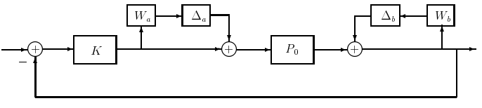
Figure 20.4: Plant with multiple uncertainties.

structure, since the two perturbations enter at different points in the system:

\[\Delta=\left[\begin{array}{cc}
\Delta_{a} & 0 \\
0 & \Delta_{b}
\end{array}\right] \ \tag{20.13}\]

Thus, there is some added information about the plant uncertainty that can- not be captured by the unstructured small-gain theorem, and in general, even if \(\|M\|_{\infty} \geq 1\) for the \(M\) that corresponds to the \(\Delta\) above, there may be no admissible perturbation that will result in unstable \((I-M \Delta)^{-1}\).

Example 20.4

Suppose that in addition to norm bounds on the uncertainty, we know that the phase of the perturbation remains in the sector \(\left[-30^{\circ}, 30^{\circ}\right]\). Again, even if \(\|M\|_{\infty} \geq 1\) for the \(M\) that corresponds to the \(\Delta\) for this system, there may be no admissible perturbation that will result in unstable \((I-M \Delta)^{-1}\).

In both of the preceding two examples, the unstructured small-gain theorem gives con- servative results.

Relating Stability Robustness to the (SISO) Nyquist Criterion

Suppose we have a SISO nominal plant with a multiplicative perturbation, and a nominally stabilizing controller \(K\). Then \(P=P_{0}(1+W \Delta)\), and the compensated open-loop transfer function is

\[P K=P_{0} K+P_{0} K W \Delta \ \tag{20.14}\]

Since \(P_{0}\), \(K\), and \(W\) are known and \(|\Delta| \leq 1\) with arbitrary phase, we may deduce from (20.14) that the "real" Nyquist plot at any given frequency \(\omega_{0}\) is contained in a region delimited by a circle centered at \(P_{0}\left(j \omega_{0}\right) K\left(j \omega_{0}\right)\), with radius \(\left|P_{0} K W\left(j \omega_{0}\right)\right|\). This is illustrated in Figure 20.5(a). Clearly, if the circle of uncertainty ever includes \(-1\), there is the possibility that the "real" Nyquist plot has an extra encirclement, and hence is unstable. We may relate this to the robust stability problem as follows. From Example 20.2, the SISO system is robustly stable by the small gain theorem if

\[\left|\frac{P_{0} K}{1+P_{0} K} W\right|<1, \quad \forall \omega \ \tag{20.15}\]

Equivalently,

\[\left|P_{0} K W\right|<\left|1+P_{0} K\right| \ \tag{20.16}\]

The right-hand side of (20.16) is the magnitude of a translation of the Nyquist plot of the nominal loop transfer function. In Figure 20.5(b), because of the translation, encirclement of zero will destabilize the system. Clearly, this cannot happen if (20.16) is satisfied. This makes the relationship of robust stability to the SISO Nyquist criterion clear.

Performance as Stability Robustness

Suppose that, for some plant model \(P\), we wish to design a feedback controller that not only stabilizes the plant (first order of priority!), but also provides some performance benefits, such as improved output regulation in the presence of disturbances. Given that something is known

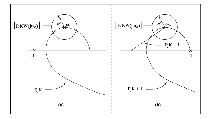
Figure 20.5: Relation of Nyquist criterion and robust stability.

about the frequency spectrum of such disturbances, the system model might look like Figure 20.6, where \(\|\xi\|_{2}<1\), and the modeling filter \(W\) can be constructed to capture frequency characteristics of the disturbance. Calculating the transfer function of this loop from \(\xi\) to \(y\), we have that \(y=(I+P K)^{-1} W \xi\). We assume that the performance specification will be met if \(\left\|(I+P K)^{-1} W\right\|_{\infty}<1\), which does not restrict the problem, since \(W\) can always be scaled to reflect the actual magnitude of the disturbance or performance specification. This formulation looks analogous to a robust stability problem, and indeed, it can be verified that the small-gain theorem applied to the system of Figure 20.7 captures the identical constraint on the system transfer function. By mapping this system into the standard form of Figure 20.3, we find that \(M=(I+P K)^{-1} W\), which is exactly the \(M\) that is needed if the small-gain condition is to yield the desired condition

Finally, plant uncertainty has to be brought into the picture simultaneously with the

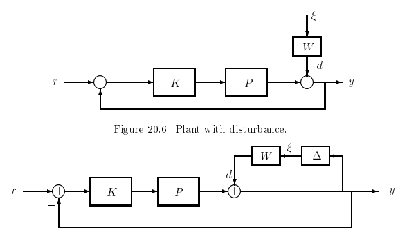
Figure 20.7: Mapping performance specifications into a stability problem.

performance constraints. This is necessary to formulate the performance robustness problem. It should be evident that this will lead to situations with block-diagonal \(\Delta\), as was obtained in the context of the last example in the previous subsection. The treatment of this case will require the notion of structured singular values, as we shall see in the next lecture.