21.2: Robust Disturbance Rejection

We will focus our discussion on one prototype problem, namely, the robust disturbance rejection problem shown in Figure 21.1. This motivates the following problem:

Robust Disturbance Rejection Projection (RP)

Find conditions on the nominal closed-loop system \((P_{o}, K)\) such that

1. \(K\) robustly stabilizes all \(P \in \Omega\), where \(\Omega=\left\{P \mid P=\left(I+\Delta_{1} W_{1}\right) P_{o}, \quad\|\Delta\|_{\infty}<1\right\}\)

2. \(\left\|(I+P K)^{-1} W_{2}\right\|_{\infty} \leq 1\) for all \(P \in \Omega\).

From Lecture 20, a performance objective in terms of the \(\mathcal{H}_{\infty}\)-norm of some closed loop map between some exogenous input \(w\), to a regulated variable \(z\), is mathematically equivalent to a robust stabilization problem with a perturbation block mapping the regulated output \(z\) to the exogenous input \(w\). Obviously, the new perturbed system is stable if and only if \(|| T_{z w} \|_{\infty} \leq 1\), which is the performance objective. Notice that if the performance objective consists of several closed loop maps, then several perturbation blocks can be introduced in exactly the same fashion.

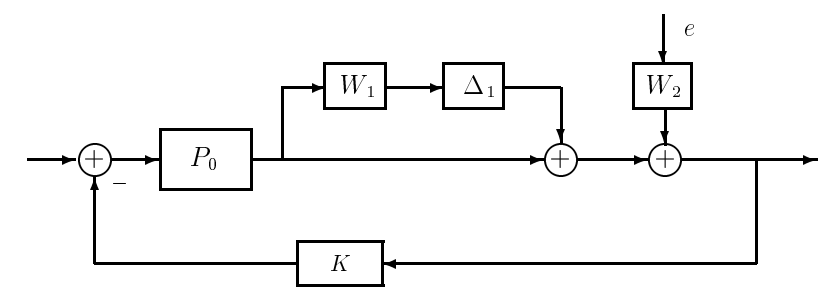
Figure 21.1: Uncertain Plant with Disturbance 

Proceeding for RP, we can "wrap" a frequency-weighted perturbation from the output to the input of interest, which results in the model of Figure 21.2. Next, we can re-arrange the system into the M-\(\Delta\) feedback form (a nominal stable \(M\) in feedback with the perturbation \(\Delta\)) as in Figure 21.3. In this case, however, there are multiple inputs and outputs to consider. We use the following procedure to generate \(M\) and \(\Delta\):

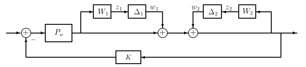
Figure 21.2: Robust Performance Model

1. Define \(w_{i}, z_{i}\) to be the output and input, respectively, of the perturbation \(\Delta_{i}\).

2. For a total of \(m\) perturbations, compute the matrix transfer function M as the map from

\[w=\left[\begin{array}{c}
w_{1} \\
\vdots \\
w_{m}
\end{array}\right] \quad \text { to } \quad z=\left[\begin{array}{c}
z_{1} \\
\vdots \\
z_{m}
\end{array}\right]\label{21.2}\]

In other words, all the \(\Delta\) blocks are removed, and the transfer functions "seen" by the blocks from each input \(w_{j}\) to each output \(z_{i}\) are calculated and used as the \((i, j)th\) element of \(M\).

3. The perturbation matrix \(\Delta\) will have the structure

\[\Delta=\left[\begin{array}{lll}
\Delta_{1} & & \\
& \ddots & \\
& & \Delta_{m}
\end{array}\right], \quad\left\|\Delta_{i}\right\|_{\infty}<1\label{21.2}\]

For a SISO system, each \(\Delta_{i}(j \omega)\) is a scalar, so that \(\Delta\) becomes a diagonal matrix with complex entries. In the MIMO case, \(\Delta\) is block-diagonal.

Example \(\PageIndex{21.1}\) (Robust Disturbance Rejection)

Applying the robust performance procedure to Figure 21.2 yields:

\[M=\left[\begin{array}{cc}
-W_{1}\left(I+P_{0} K\right)^{-1} P_{0} K & -W_{1}\left(I+P_{0} K\right)^{-1} P_{0} K \\
W_{2}\left(I+P_{0} K\right)^{-1} & W_{2}\left(I+P_{0} K\right)^{-1}
\end{array}\right]\label{21.3}\]

The transfer functions on the diagonal are identical to those in the single-block robust stability and disturbance-rejection problems, respectively, while the off-diagonal terms account for the interaction between the two constraints. Having found the appropriate \(M\) and \(\Delta\), we have thereby reduced the robust performance problem to a stability problem for the system of Figure 21.3.

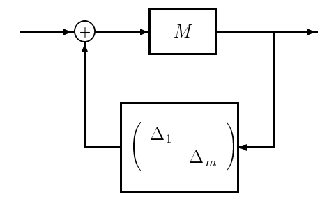
Figure 21.3: M- \(\Delta\) Feedback Form 

A sufficient condition for robust stability is given by the small gain theorem, namely,

\[\begin{aligned}
&\sigma_{\max }[M(j w)] \sigma_{\max }[\Delta(j w)] \leq \gamma<1\\
&\text { for all } w \text { . }
\end{aligned}\nonumber\]

Since \(\Delta\) is norm bounded by one, this condition translates to \(\|M\|_{\infty} \leq \gamma\). This condition, however, is far from necessary since \(\Delta\) has a block diagonal structure.