4.1: Stability of the Closed-Loop System
- Page ID
- 24402

Closed-Loop Stability
Ensuring the stability of the closed-loop is the first and foremost control system design objective. Even though the physical plant, \(G(s)\), may be stable, the presence of feedback can cause the closed-loop system to become unstable, as in the case of higher order plant models.
The standard block diagram of a single-input single-output (SISO) feedback control system (Figure 4.1.1) includes a plant, \(G(s)\), a controller, \(K(s)\), and a sensor, \(H(s)\), where \(H\left(s\right)=1\) is assumed.
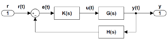
The overall system transfer function from input, \(r(t)\), to output, \(y(t)\), is given as: \[T(s)=\frac{KG(s)}{1+KGH(s)} \nonumber \]
The determination of stability is based on the closed-loop characteristic polynomial: \[\Delta (s,K)=1+KGH(s). \nonumber \]
In particular, let \(G\left(s\right)=\frac{n\left(s\right)}{d\left(s\right)}\); then, assuming a static controller: \(K(s)=K\), the closed-loop characteristic polynomial is given as: \[\Delta (s,K)=d(s)+Kn(s) \nonumber \]
Alternatively, assuming a dynamic controller, \(K\left(s\right)=\frac{n_C\left(s\right)}{d_C\left(s\right)}\), the characteristic polynomial is given as: \[\Delta (s)=d(s)d_{C} (s)+n(s)n_{C} (s) \nonumber \]
Stability Determination by Algebraic Methods
The stability of the characteristic polynomial is determined by algebraic methods that characterize its root locations based on the coefficients of the polynomial. In the following, we assume that \(\Delta (s)\) is an \(n\)th order polynomial expressed as:
\[\Delta (s)=s^{n} +a_{1} s^{n-1} +\ldots +a_{n-1} s+a_{n} \nonumber \]
Necessary Condition. A necessary condition for stability of the polynomial is that coefficients \(a_i, \; i=1,2,\cdots,n\), are all nonzero and are positive, i.e., \(a_i>0\).
Sufficient Condition. A sufficient condition for polynomial stability is obtained through the application of the following equivalent criteria:
The Hurwitz Criterion
The \(n\)th order polynomial, \(s^n+a_1s^{n-1}+\dots +a_n\) is stable, i.e., has its roots in the open left-half plane (OLHP), if and only if the following determinants assume positive values:
\[\left|a_{1} \right|,\; \; \left|\begin{array}{cc} {a_{1} } & {a_{3} } \\ {1} & {a_{2} } \end{array}\right|,\; \; \left|\begin{array}{ccc} {a_{1} } & {a_{3} } & {a_{5} } \\ {1} & {a_{2} } & {a_{4} } \\ {0} & {a_{1} } & {a_{3} } \end{array}\right|,\ldots \nonumber \]
The Routh’s Criterion
The \(n\)th order polynomial, \(s^n+a_1s^{n-1}+\dots +a_n\) is stable, i.e., has its roots in the open left-half plane (OLHP), if and only if all entries in the Routh's array are positive.
\[\begin{array}{c} {\begin{array}{c} {s^{n} } \\ {s^{n-1} } \\ {\vdots } \\ {} \\ {s^{1} } \\ {s^{0} } \end{array}} \end{array}\left|\begin{array}{c} {\begin{array}{cccc} {1} & {a_{2} } & {\ldots } & {} \\ {a_{1} } & {a_{3} } & {\ldots } & {} \\ {b_{1} } & {b_{2} } & {\ldots } & {} \\ {c_{1} } & {c_{2} } & {\ldots } & {} \\ {\ldots } & {} & {} & {} \\ {\ldots } & {} & {} & {} \end{array}} \end{array}\right. \nonumber \]
The first two rows in the Routh's array are filled by alternating the coefficients of the polynomial. The entries appearing in the third and subsequent rows are computed as follows:
\(b_{1} =-\frac{1}{a_{1} } \left|\begin{array}{cc} {1} & {a_{3} } \\ {a_{1} } & {a_{2} } \end{array}\right|,\; \; b_{2} =-\frac{1}{a_{3} } \left|\begin{array}{cc} {a_{2} } & {a_{4} } \\ {a_{3} } & {a_{5} } \end{array}\right|,\; \; c_{1} =-\frac{1}{b_{1} } \left|\begin{array}{cc} {a_{1} } & {a_{3} } \\ {b_{1} } & {b_{2} } \end{array}\right|\), etc.
The Routh’s stability criterion states that the number of unstable roots of the polynomial equals the number of sign changes in the first column of the Routh’s array.
Stability Determination for Low-Order Polynomials
Low-order polynomials (i.e., polynomials of degree \(n=2,\; 3\)) are often encountered in model-based control system design. The Routh or Hurwitz can be simplified when applied to such polynomials.
The stability criteria for second and third-order polynomials are given below:
Second-order polynomial: (\(n=2\)): \(\, a_{1} >0,\; \, a_{2} >0\).
Third-order polynomial: (\(n=3\)): \(\, a_{1} >0,\quad a_{2} >0,\quad a_{3} >0,\quad a_{1} a_{2} -a_{3} >0.\)
Controller Gain Selection
The stability conditions can be used to determine the range of controller gain, \(K\), to ensure that the roots of the closed-loop characteristic polynomial, \(\Delta (s,K)\), lie in the open left-half plane (OLHP).
Let \(G\left(s\right)=\frac{K}{s\left(s+2\right)}\), \(H\left(s\right)=1\); then, \(\Delta (s,K)=s^{2} +2s+K\). By using the above stability criteria, \(\Delta (s)\) is stable for \(K>0\).
Let \(\Delta (s,K)=s^{3} +3s^{2} +2s+K\). By using the above stability criteria, \(\; \Delta (s)\) is stable if the following conditions are met: \(K>0\) and \(6-K>0\). Accordingly, the range of \(K\) for closed-loop stablity is given as \(0<K<6\).
The simplified model of a small DC motor is given as: \(\frac{\theta (s)}{V_a (s)} =\frac{10}{s(s+6)} .\)
A PID controller for the motor model is defined as: \(K(s)=k_ p +k_ d s+\frac{k_ p }{s}\). The closed-loop characteristic polynomial is given as:
\[\Delta (s)=s^{2} (s+6)+10(k_ d s^{2} +k_ p s+k_{i} )=s^{3} +(6+10k_ d )s^{2} +10k_ p s+10k_{i} . \nonumber \]
The constraints on the PID controller gains to ensure the stability of the third-order polynomial are given as:
\[k_ p ,\; k_{i} ,\; 6+10k_ d >0 \nonumber \]
\[k_ p (6+10k_ d )-k_{i} >0 \nonumber \]
We may choose, e.g., \(k_ p =1,\, k_ i =1,\, k_ d =1\) to meet the stability requirements.
Stability Determination from Frequency Response Plots
The frequency response function of the loop gain, \(KGH\left(j\omega \right)\), can be used to determine the stability of the closed-loop system. In particular, the root condition on the closed-loop characteristic polynomial implies: \(1+KGH\left(j\omega \right)=0\), or \(KGH\left(j\omega \right)=-1\).
Hence stability of the closed-loop system can be inferred from the frequency response of \(KGH\left(j\omega \right)\), relative to the \(1\angle \pm 180{}^\circ\) point on the complex plane. The stability determination is performed using the following relative stability criteria:
The gain margin (GM) denotes the factor by which the loop gain,\(\ \left|KGH\left(j\omega \right)\right|\), can be increased without compromising the closed-loop stability.
The GM is computed as: \(GM=-{\left|KGH\left(j{\omega }_{pc}\right)\right|}_{dB},\) where \({\omega }_{pc}\) denotes the phase crossover frequency defined by \(\angle KGH\left(j\omega \right)=-180{}^\circ\).
A positive value of GM denotes closed-loop stability.
The phase margin (PM) denotes the additional phase that can be added by the controller to \(\angle KGH\left(j\omega \right)\) without compromising the closed-loop stability.
The PM is computed as: \(PM=\angle KGH\left(j{\omega }_{gc}\right)+180{}^\circ ,\) where \({\omega }_{gc}\) denotes the gain crossover frequency defined by \({\left|KGH\left(j{\omega }_{gc}\right)\right|}_{dB}=0dB\).
A positive value of PM denotes closed-loop stability. Additionally, PM represents a measure of dynamic stability; hence adequate PM is desired to suppress oscillations in the output response.
To proceed further, assume that the loop transfer function, \(KGH\left(s\right)\), has \(m\) zeros and \(n\) poles. Then,
- For low-order models (\(n\le 2)\), the loop gain, \(KGH\left(s\right)\), displays an infinite GM.
- GM is finite for \(n-m>2\) and may be so for \(n-m=2\).
The gain crossover occurs when \({\left|KGH\left(j0\right)\right|}_{dB}>0dB\); hence PM become relevant only in that case.
Stability Determination on Bode Plot
On the Bode magnitude plot the gain crossover frequency, \({\omega }_{gc}\), is indicated as the magnitude plot crosses the \(0dB\) line. The Bode phase plot at that frequency reveals the phase margin as: \(PM=\angle KGH\left(j{\omega }_{gc}\right)+180{}^\circ\).
On the Bode phase plot, phase crossover frequency, \({\omega }_{pc}\), is indicated as the phase plot crosses the \(-180{}^\circ\) line. The magnitude plot at that frequency reveals the gain margin as: \(GM=-{\left|KGH\left(j{\omega }_{pc}\right)\right|}_{dB}\).
The relative stability margins can be obtained in the MATLAB Control Systems Toolbox by using the ‘margin’ command. When invoked the command produces a Bode plot with stability margins indicated.
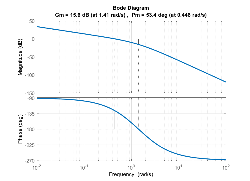
Let \(KG\left(s\right)=\frac{K}{s(s+1)(s+2)}\); the Bode magnitude and phase plots for \(K=1\) are shown in Figure 4.1.2.
The Bode magnitude plot displays a \(15.6\;dB\) gain margin, i.e., the controller gain can be increased by a factor of \(6\:(15.6\,dB)\) before losing stability of the closed-loop system.
The Bode phase plot displays a \(53.4{}^\circ\) phase margin, which indicates closed-loop stability; further, it corresponds to \(\zeta \cong 0.55\) for the closed-loop system, which indicates adequate dynamic stability.
Stability Determination on Nyquist Plot
On the Nyquist plot, the gain crossover is indicated when the Nyquist plot enters the unit circle, whereas phase crossover is indicated when the Nyquist plot crosses the negative real-axis.
Thus, GM is positive if the real-axis crossing is to the right of \(-1+j0\) point. The PM is positive if \(KGH\left(j\omega \right)\) magnitude drops below unity in the third quadrant.
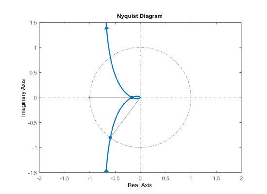
Let \(KG\left(s\right)=\frac{K}{s(s+1)(s+2)}\); the Nyquist plot for \(K=1\) is shown in Figure 4.1.3.
The Nyquist plot crosses the real axis at \(s=-0.165\), which corresponds to \(GM=6\).
The Nyquist plot enters the unit circle at an angle of \(53^\circ\) from the negative real axis that indicates the phase margin.
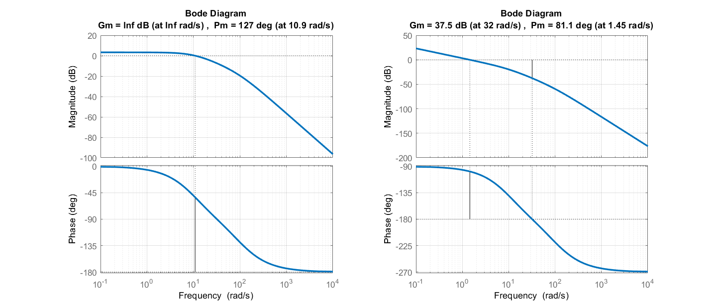
The model of a small DC motor, including an amplifier with a gain of 3 is given as: \(\frac{\omega (s)}{V_a (s)} =\frac{1500}{(s+100)(s+10)+25}\).
The relative stability margins for the DC motor model are given as: \(GM=\infty ;PM=127{}^\circ\) (Figure 4.1.4).
Assume that the motor is used in a position control application, so that the plant transfer function is given as: \(\frac{\theta (s)}{V_a (s)} =\frac{1500}{s\left[(s+100)(s+10)+25\right]}\).
The corresponding relative stability margins are given as: \(GM=37.5\ dB;\ PM=81.1{}^\circ\) (Figure 4.1.4).