2.8: Fitting ODE parameters to data using Excel- Using regression to fit complex models in Excel

Section 8. Fitting ODE parameters to data using Excel: Using regression to fit complex models in Excel

Note: Video lecture available for this section!

Authors: Anthony Campbell, Victoria Cardine, David Hines, Stephen Kerns /Date Revised: 14th September 2007

Stewards: Jeff Byrd, Khek Ping Chia, John Cruz, Natalie Duchene, Samantha Lyu

Introduction

One of the most important abilities of an engineer is to model measured values of a system. Modeling of a system aids in optimizing objectives, as well as predicting future operations. This can be especially helpful when changes cannot be immediately implemented. In general modeling terms, a set of data can always fit a set of variables. However, an excessive number of degrees of freedom usually exist, creating multiple solutions. Therefore, the physical significance of the variables is an important consideration.

As time proceeds, various values may need to be changed to accommodate variations within the system. The following sections will discuss the use of Microsoft Excel© as a tool to adjust the values of variables given a set of experimental data. The models presented below take into account the design equations of the system being modeled, and the rate laws, where applicable.

Adding in the Solver Application in Excel 2007

In order to use "Solver" in Excel 2007, one must first add the Excel tool-pack. To add the tool-pack, follow these instructions:

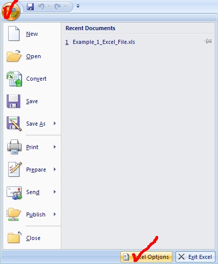
• Click on the Microsoft Office symbol at the top left corner of the screen
• Click on “Excel options” at the bottom right corner of the drop box
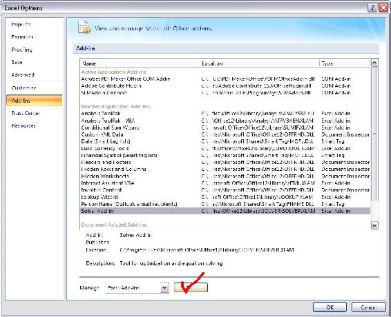
• Click on “Add-Ins” in the left hand column
• Click on the “Solver Add-In” option at the bottom of the list
• Click on “GO” at the bottom right corner
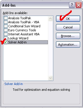
• Check the “Solver Add-in” box at the bottom of the list
• Click on “OK” at the top of the right column

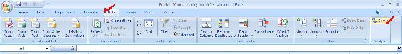
To access Solver, click on the “Data” tab at the top of the screen. The Solver tool is located in the "Analysis" box on the right side of the screen.

The user interface of Excel 2007 differs from those of previous versions. The following images illustrate the process just described.

In order to use the Solver function, click on Data and then the Solver button in the Analysis box.

NOTE: If using Microsoft Office 2003, the Solver Application can be added by clicking on the "Tools" tab at the top of the screen. The same directions can be followed after this step.

NOTE: If you receive an error message while trying to access Solver, it may already be added in Excel. Uninstall Solver (by following the same steps, but unchecking "Solver Add-in") then reinstall it.

Adding in the Solver Application in Excel 2008

Excel 2008 for Macs does not come with the solver add-in. The software can be downloaded at Solver.com

This solver application requires Excel 12.1.2. If this is not the current version of Excel being used, it can be updated by running Microsoft AutoUpdate or by opening excel, going to help and then clicking on "Check for Updates". Make sure when updating Excel to close all Microsoft Applications.

This application allows the user to have a solver program that can be opened and used while running Excel. It works the same way as the solver add-in.

Using Excel Solver to Fit ODE Parameters

Excel Solver is a tool that can be used to fit function variables to given experimental data. The following process can be used to model data:

• Define the data set by entering values into an Excel spreadsheet
• Define the model that you want to fit to the data
• Define the sum of least squares in one of the spreadsheet blocks
• In Solver, have Excel minimize the sum of least squares by varying the parameters in the model

Accurate modeling is dependent on two factors; initial values and verifying results.

Initial values: As stated in the introduction, many data fitting problems can have multiple “solutions”. In numerical methods, given a set of initial parameters the data will converge to a solution. Different initial values can result in differing solutions. Therefore, if the initial values are not set by the problem statement, multiple initial guesses should be entered to determine the “best” value for each variable.

Verification of curve fit: When fitting a curve to given data points, it is important to verify that the curve is appropriate. The best way to do this is to view the data graphically. It is fairly simple to use the Chart tool to graph the data points. Adding a trend line will show the mathematical relationship between the data points. Excel will generate a function for the trend line and both the function and the R-squared value can be shown on the plot. This can be done by clicking “Options” next to “Type” of trend and checking the empty boxes that are labeled “Display equation on chart” and “Display R-squared value on chart”.

There are various types of trendlines that can be chosen for your given data points. Depending on the trend that you may see, you might want to try a few of the options to obtain the best fit. Sometimes the squared residual value will be better for a certain type of trend, but the trend is not necessarily “correct”. When you have obtained sample data, be aware of the trend you should be seeing before fitting a certain trend type to the data points (if this is possible). The polynomial trend type gives you the option to change the order of the equation.

Typically, you will not acquire a squared residual value of zero. This value is a simple analysis of the error between the trend line, and the actual data. Once the function and squared residual values are generated, you can begin to evaluate the generated solution.

During your solution analysis, it is important to check for variables or parameters that may be unnecessarily influencing the data. Excel can generate a "best" solution, which is not correct due to background calculations or Excel's misinterpretation of the modeled system. To assess this possibility, you can graph data generated by using the solved for variables against the given data.

Additional information about the Excel Solver Tool can be found in Excel Modeling.

Worked out Example 1: Mass Balance on a Surge Tank

In this example we will walk through the scenario in which you want to model a non-heated surge tank in Microsoft Excel©. This model would be very critical in a process where smooth levels of process flow are required to maintain product specifications. Therefore, an engineer would like to know whether they will need to periodically refill or drain the tank to avoid accidents. Let's look at this simple example:

Problem statement:

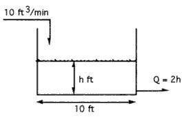
Suppose water is being pumped into a 10-ft diameter tank at the rate of 10 ft3/min. If the tank were initially empty, and water were to leave the tank at a rate dependent on the liquid level according to the relationship Qout = 2h (where the units of the constant 2 are [ft2/min], of Q are [ft3/min], and of h are [ft]), find the height of liquid in the tank as a function of time. Note that the problem may be, in a way, over specified. The key is to determine the parameters that are important to fit to the experimental surge tank model.

Solution:

The solution with fitted parameters can be found here: Surge tank solution This Excel file contains this scenario, where given the actual data (the height of the liquid at different times), the goal is to model the height of the liquid using an ODE. The equations used to model h(t) are shown and captioned. In order to parameterize the model correctly, Solver was used to minimize the sum of the least square differences at each time step between the actual and model-predicted heights by changing the parameters' values. The model predicts the actual height extremely well, with a sum of the least squared differences on the order of 10^-5. A graph showing the modeled and actual height of the tank as a function of time is included as well.

Worked out Example 2: Fitting a heated surge tank model(a heated CSTR) parameters to data in Excel

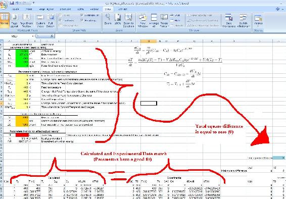
Problem Introduction: In this example we will analyze how we can fit parameters used for modeling a heated CSTR to data stored in Excel. The purpose of this problem is to learn how to vary ODE parameters in Excel in order to achieve a square difference between the calculated and experimental data of zero. Some questions to consider are, “How do I model this? Is this a first order ODE? Are there any coupled ODE's? How many variables need to be considered?" This example will use an Excel file to help you in this process.

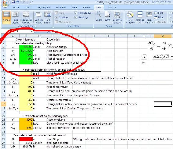
Problem Statement: Download the heated CSTR problem file.CSTR Problem Take the experimental data produced from the heated CSTR model in the Excel spreadsheet*. You are modeling a heated CSTR. It would be wise and is highly recommended to review both the heated CSTR problem and a wiki on using Excel's solver.

You know this is a heated CSTR...

2. Numerically solve the ODEs through modifying the given wrong set of parameters.
3. While changing the parameters, use Excel to calculate the error between the calculated model and the experimental data.
4. Use the Excel solver function to solve for some of the parameters to minimize error to less than 5%
5. How would your approach be different if our heat transfer area needed to be as small as possible due to capital constraints? Explain.
6. How would your approach be different if our mass feed rate has to be in the range of 3-3.5 kg/s? Explain.

Problem Solution: The solution with fitted parameters can be found here.CSTR Solution

With the model and data given in the example the error must first be defined. Here there error is the squared residual or [(model observation at time i)-(data observation at time i)]^2 over (all i).

Chemical engineering intuition must be used to reasonably approximate some variables. In real life we would double check that "parameters normally known, but erroneous" are correct. (Due to problem constraints, we will assume these are accurate, but a true chemical engineer would check regardless). We must now modify "parameters often needing fitting". For part 3, we can modify the parameters as shown in the solution.

The original parameters have been modified to produce an error of zero.

If we have restrictions on heat exchange area then we should try to fit the "heat transfer coefficient and area" as low as possible. Likewise, if we have restrictions on feed rate, we must keep this above 4 while fitting other parameters as best as possible to achieve a small error. These have certain industrial applications as costing of heat exchangers and limitations on mass flow rates need to be modeled before a reactor design is implemented.

Side Note: The example above assumes a first order rate law. This is not always the case. To change the equations to fit a new rate law, one must derive a new dCa/dt equation and dT/dt using their knowledge of reactor engineering. Once the new equations are derived write the formula in an excel format in our dCa/dt and dT/dt column and then drag it to the end of the column. All other columns should stay the same.

Sage's Corner

A brief narration for a better understanding of Example 1 - Surge Tank Model and tips for effectively picking a model equation can be found here: video.google.com/googleplayer.swf?docId=70222262469581741
A copy of the slides can be found here:

Unnarrated Slides

An example of fitting an ODE parameter to data using excel - based on a simple radioactive decay rate ODE: video.google.com/googleplayer.swf?docId=8229764325250355383
A copy of the slides can be found here: Unnarrated Slides
A copy of the excel file can be found here: Excel File

An example of modelling a reaction rate ODE with rate constant and rate order variable parameters:
video.google.com/googleplayer.swf?docId=-4220475052291185071
A copy of the slides can be found here: Unnarrated Slides
A copy of the excel file can be found here: Excel File

References

Holbert, K.E. "Radioactive Decay", 2006, ASU Department of Electrical Engineering, Online: October 1, 2007. Available www.eas.asu.edu/~holbert/eee460/RadioactiveDecay.pdf