6.8: Modeling and PID Controller Example - Cruise Control for an Electric Vehicle

Introduction

Controls principles developed in this course can be applied to non-chemical engineering systems such as automobiles. Some companies, such as NAVTEQ, are developing adaptive cruise control products that use information about the upcoming terrain to shift gears in a more intelligent manner which improves speed regulation and fuel economy. This case study will examine the basics of develop a speed controller for an electric vehicle.

An electric vehicle was chosen for the following reasons:

• Electric vehicles are interesting from an engineering perspective and may become a reality for consumers in the future
• Torque produced by an electric motor is instantaneous (for all practical purposes). Thus actuator lag can be ignored, simplifying the development of said controller.
• Some electric vehicles feature motors directly integrated into the hub of the drive wheel(s). This eliminates the need for a transmission and simplifies vehicle dynamics models.

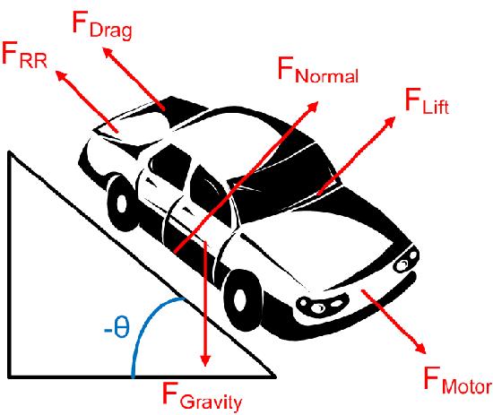
Forces

As shown in the free body diagram below, there are six forces acting on the vehicle:

1. Rolling Resistance
2. Aerodynamic Drag
3. Aerodynamic Lift
4. Gravity
5. Normal
6. Motor

Figure 1: A free body diagram of the forces acting on the vehicle. \(-\theta\) is used to denote the grade of the road such that a positive value of \(\theta\) corresponds to the vehicle traveling uphill.

Rolling Resistance

Rolling resistance is due the tires deforming when contacting the surface of a road and varies depending on the surface being driven on. It can be model using the following equation:

\[F_{R R}=C_{r r 1} v+C_{r r 2} F_{N} \nonumber \]

The two rolling resistance constants can be determined experimentally and may be provided by the tire manufacture. is the normal force.

Aerodynamic Drag

Aerodynamic drag is caused by the momentum loss of air particles as they flow over the hood of the vehicle. The aerodynamic drag of a vehicle can be modeled using the following equation:

• is the density of air. At 20°C and 101kPa, the density of air is 1.2041 kg/m³.
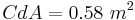
• is the coefficient of drag for the vehicle times the reference area. Typical values for automobiles are listed here.
• is the velocity of the vehicle.

Aerodynamic Lift

Aerodynamic lift is caused by pressure difference between the roof and underside of the vehicle. Lift can be modeled using the following equation:

• is the density of air. At 20°C and 101kPa, the density of air is 1.2041 kg/m³.
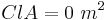
• is the coefficient of lift for the vehicle times the reference area.
• is the velocity of the vehicle.

Gravity

In the diagram above, there is a component of gravity both in the dimension normal to the road and in the dimension the vehicle is traveling. Using simple trigonometry, the component in the dimension of travel can be calculated as follows:

\[F_{G, t r a v e l}=m g \sin (-\theta) \nonumber \]

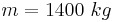
• \(m\) is the mass of the vehicle.
• \(g\) is the acceleration due to gravity.

Normal Force

The normal force is the force excerted by the road on the vehicle's tires. Because the vehicle is not moving up or down (relative to the road), the magnitude of the normal forces equals the magnitude of the force due to gravity in the direction normal to the road.

• \(m\) is the mass of the vehicle.
• \(g\) is the acceleration due to gravity.

Motor

The torque produced by an electric motor is roughly proportional to the current flowing through the stater of the motor. In this case study, the current applied to the motor will be controlled to regulate speed. Applying a negative current will cause the vehicle to regeneratively brake.

\[ \tau=k_{\text {motor}} I \nonumber \]

\[F_{M}=\frac{\tau}{r}=\frac{k_{\text {motor }} I}{r} \nonumber \]

• is the torque produced by the motor.
• is the current flowing through the motor.
• is the radius of the tire.
• is a constant.

Newton's Second Law

Using Newton's Second Law, a differential for the vehicle's speed can be obtained.

\[\begin{align*} m a &=\sum F \\[4pt] &=F_{M}-F_{d r a g}-F_{R R}+F_{G, \text {travel}} \end{align*} \nonumber \]

Substituting in the expressions for various forces detailed above yields the following:

Further substituting the expression for normal forces yields the following:

Substituting for results in the following:

Grouping like turns results in the following:

In order to simply the remaining analysis, several constants are defined as follows:

\[\beta=r C_{r r 1} \nonumber \]

\[\gamma=r C_{r r 2} m g \cos (-\theta)-r m g \sin (-\theta) \nonumber \]

Substituting these into the differential equation results in the following expression:

\[\frac{d v}{d t}=\frac{\tau-\alpha v^{2}-\beta v-\gamma(\theta)}{m r} \nonumber \]

It is important that \(\theta\) (and thus also \(\gamma\)) is a function of vehicle position.

PID Controller

One way to regulate vehicle speed is to control the torque generated by the electric motor. If the motor torque is greater than the resistive torque acting on the vehicle (a summation of aerodynamic drag, rolling resistance, etc.) the vehicle will accelerate. If the motor torque is less than the resistive torque, the vehicle will slow down.

Expression for Phase Current

For an electric motor, the phase current flowing through the motor is proportional to the torque produced. Thus one strategy for controlling the vehicles speed is to controller the motor phase current.

Using a PID controller architecture, the expression for motor current is the following:

\[I=K_{c}\left(v_{s e t}-v\right)+\frac{1}{\tau_{I}} \int(v-v_{set}) d t+\tau_{D} \frac{d\left(v_{s e t}-v\right)}{d t}+C_{offset} \nonumber \]

Differential Equation for Velocity

Substituting this expression into the differential equation for vehicle position results in the following:

\[\dfrac{dv}{dt} = \frac{k_{motor}[K_{c}(v_{set}-v) + \frac{1}{\tau_{I}} \int {(v_{set}-v)dt} + \tau_{D} \frac{d(v_{set}-v)}{dt} + C_{offset}]- \alpha v^2 - \beta v - \gamma(\theta)}{m r} \nonumber \]

Defining another variable \(x_1\) allows for the removal of the integral from the expression.

\[\frac{d x_{1}}{d t}=v_{s e t}-v \nonumber \]

\[\frac{d v}{d t}=\frac{k_{\text {motor}}\left[K_{c}\left(v_{\text {isct }}-v\right)+\frac{x_{1}}{\tau_{l}}+\tau_{D} \frac{d\left(v_{a=t}-v\right)}{d t}+ C_{offset} \right]-\alpha v^{2}-\beta v-\gamma(\theta).}{m r} \nonumber \]

If all changes in \(v_{set}\) are gradual then \(\frac{d v_{set}}{d t} \approx 0\). Applying this simplification results in the following expression:

\[\frac{d v}{d t}=\frac{k_{\text {motor }}\left[K_{c}\left(v_{\text {set }}-v\right)+\frac{x_{1}}{\tau_{1}}-\tau_{D} \frac{d v}{d t}+C_{\text {offset }}\right]-\alpha v^{2}-\beta v-\gamma(\theta)}{m r} \nonumber \]

Using a little algebra, an expression for can be obtained as follows:

\[\frac{d v}{d t}=\frac{k_{\text {motor}} K_{c}\left(v_{\text {set}}^{k_{\text {motor}}} x_{1} | k_{\text {motor}} C_{\text {cffses}}^{2}\right)^{\alpha}(\theta)}{\dot{k}_{\text {motor}} l_{L}+mr} \nonumber \]

Find Fixed Point

The fixed point can be obtained by setting the derivatives to zero and solving the system of equation.

System of Equations:

\[\frac{d v}{d t}=\frac{k_{\text {meclor }} K_{c}\left(v_{\text {sel }}-v\right)+\frac{k_{\text {motor }}}{\tau_{I}} x_{1}+k_{\text {melur }} C_{v \int j s \leq \iota}-\alpha v^{2}-\beta v-\gamma(\theta)}{k_{\text {motor }} t_{D}+m r}=0 \nonumber \]

\[\frac{x_{1}}{d t}=v_{s e t}-v=0 \nonumber \]

Solution

\[x_{1}=\frac{\left.-\tau_{I}\left(k_{\text {motor}} C_{\text {offset}}-\alpha v_{\text {set}}^{2}-\beta v_{\text {set}}-\gamma(\theta)\right]\right)}{k_{\text {motor}}} \nonumber \]

\[v=v_{s e t} \nonumber \]

As expected, a fixed point exists when the set velocity equals the actual velocity of the vehicle.

Linearize System of ODEs

Before the stability of the system can be (easily) examined, the system must be linearized around a fixed point.

Note: To simply the matrix expressions in section the following notation will be used:

\[y_{i}^{\prime}=\frac{d y_{i}}{d t} \nonumber \]

Overall a linearized system of ODEs has the following form:

\[\left[\begin{array}{c}
y_{1}^{\prime} \\
y_{2}^{\prime} \\
\vdots \\
y_{n}^{\prime}
\end{array}\right]=\mathbf{J}\left[\begin{array}{c}
y_{1} \\
y_{2} \\
\vdots \\
y_{n}
\end{array}\right]+\left[\begin{array}{c}
k_{1} \\
k_{2} \\
\vdots \\
k_{n}
\end{array}\right] \nonumber \]

The first step of linearizing any system of ODEs to calculate the Jacobian. For this particular system, the Jacobian can be calculated as follows:

\[\mathbf{J}=\left[\begin{array}{cc}
\frac{\partial v^{\prime}}{\partial v} & \frac{\partial v^{\prime}}{\partial x_{1}} \\
\frac{\partial x_{1}^{\prime}}{\partial v} & \frac{\partial x_{1}^{\prime}}{\partial x_{1}}
\end{array}\right]=\left[\begin{array}{cc}
\frac{-k_{m o t o r} K_{c}-m r[2 \alpha v+\beta]}{m r+k_{m o t o r} \tau_{D}} & \frac{k_{\text {motor }}}{t_{l}\left(m r+k_{\text {motor }} \tau_{D}\right)} \\
-1 & 0
\end{array}\right] \nonumber \]

The Jacobian is then evaluated at the fixed point:

\[\mathbf{J}=\left[\begin{array}{cc}
\frac{-k_{\text {motor }} K_{c}-m r\left[2 \alpha v_{\text {set }}+\beta\right]}{m r+k_{\text {motor }} \tau_{D}} & \frac{k_{\text {motor }}}{t_{I}\left(m r+k_{\text {motor }} \tau_{D}\right)} \\
-1 & 0
\end{array}\right] \nonumber \]

The next step if to calculate the vector of constants. For this particular system, said vector can be calculated as follows:

\[\left[\begin{array}{c}
k_{v} \\
k_{x_{1}}
\end{array}\right]=\left[\begin{array}{c}
\frac{\left.-\left(-k_{\text {motor}} K_{c}-2 \alpha v_{s e t}-\beta\right]\right) v_{s e t}}{\left(m r+k_{\text {motor}} \tau_{D}\right)}+\frac{\left.\left(k_{\text {motor}} C_{\text {offset}}-\alpha v_{\text {set}}^{2}-\beta v_{\text {set}}-\gamma(\theta)\right]\right)}{\left(m r+k_{\text {motor}} \tau_{D}\right)} \\
v_{\text {set}}
\end{array}\right] \nonumber \]

Combining the Jacobian and vector of constants results in the following linearized system:

\[\left[\begin{array}{l}
v^{\prime} \\
x_{1}^{\prime}
\end{array}\right]=\mathbf{J}\left[\begin{array}{l}
v \\
x_{1}
\end{array}\right]+\left[\begin{array}{l}
k_{v} \\
k_{x_{1}}
\end{array}\right] \nonumber \]

Stability Analysis

To assess the stability of the controller, the eigenvalues of the Jacobian in the linearized systems of ODEs can be examined. In general, an eigenvalue (lambda) is the solution to the following equation:

\[|\mathbf{J}-\lambda \mathbf{I}|=0 \nonumber \]

Using a computer to solve said equation, the eigenvalues of this particular system can be found to be the following:

For the system to be stable, the real component of all eigenvalues must be non-positive. The following inequality must be true for a stable controller:

For the system to not oscillate, the imaginary component of all eigenvalues must be zero. The following inequality must be true for a non-oscillating controller:

\[\tau_I (k_{motor}^2 K_c^2 \tau_I+2 k_{motor} K_c \tau_I \beta+4 k_{motor} K_c \tau_I \alpha v_{set}+\beta^2 \tau_I+4 \beta \tau_I \alpha v_{set}+4 \alpha^2 v_{set}^2 \tau_I-4 k_{motor} mr-4 k_{motor}^2 t_D) \nonumber \]

Interestingly, neither of these criteria depend on the grade of the road (θ). However, during the analysis, it was assumed that θ is constant. For most roads, this is not the case; θ is actually a function of vehicle position. In order to add this additional level of detail, the original system of ODEs needs to be revised:

\[\frac{d v}{d t}=\frac{k_{\text {motor}} K_{c}\left(v_{\text {set}}, v\right)\left|k_{\text {motor}} x_{1}\right| k_{\text {motor}} C_{\text {offset}}}{k_{\text {motor}} l_{D}+\pi u r} \nonumber \]

\[\frac{d x_{1}}{d t}=v_{set}-v \nonumber \]

\[\frac{d s}{d t}=v \nonumber \]

\[\theta=f(s) \nonumber \]

Unfortunately for any normal road, the grade is not a simple (or even explicate) function of position (s). This prevents an in depth analytical analysis of stability. However for a very smooth road with very gradual changes in grade, the stability of the controller should be unaffected.

Example Electric Vehicle

Simulating the system also for other properties of the controller to be examined. This section presents the results from simulating a specified fictitious electric vehicle.

Parameters

For the fictitious electric vehicle simulated in this analysis, the following parameters were used. These parameters are roughly based on the parameters one would expect to see in a typical electric automobile.

Root Locus Plots

Using the parameters above, Root Locus Plots of the system were constructed to numerically explore the stability. The following controller constants were used when constructing the plots:

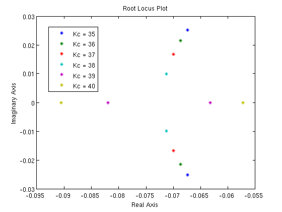
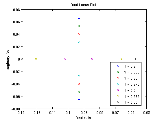
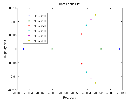
These Root Locus plots show that the controller with said constants is both stable and does not oscillate.

Phase Portrait

A phase portrait of the system with the following parameters was also constructed:

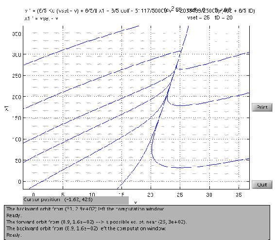
The phase portrait shows that the system is both stable and does not oscillate, as predicted by the Root Locus plots.

Driving Simulation on Level Terrain

The vehicle was simulated starting at 10 m/s and accelerating to 25 m/s via cruise control on level terrain (). For this simulation, the following constants were used:

\[C_{o f f s e t}=146 \approx \frac{\alpha v_{s e t}^{2}+\beta v_{s e t}+\gamma(\theta=0)}{k_{m o t o r}} \nonumber \]

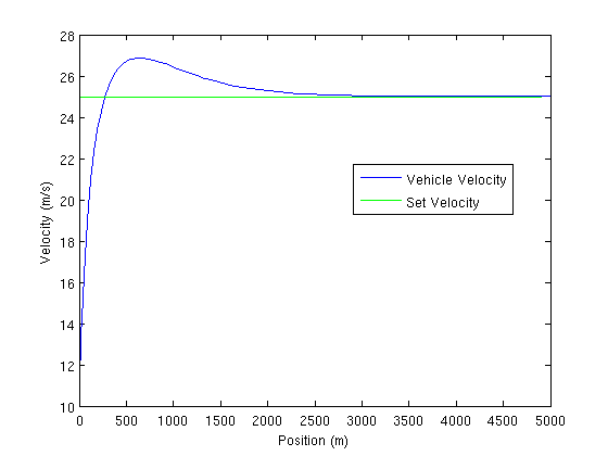
Interestingly this graph shows oscillation, despite the Root Locus plots and phase diagrams. It is important to remember, however, that the Root Locus plot and stability methods involve linearizing the system. It is possible the linearized system is not a good approximation of the system.

It is also important to remember that this particular example involves a large set point change, which can induce oscillations in certain systems.

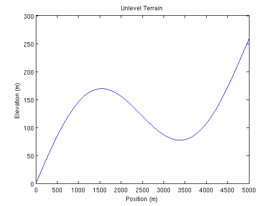
Driving Simulation on Unlevel Terrain

In order to explore how the controller behaves on a road with a non-zero grade, a route with hills was constructed from the following equation, where h is elevation and s is position.:

\[h=100 \sin \left(\frac{s}{250 \pi}\right)+\frac{s}{2000} \nonumber \]

The vehicle was simulated driving said road starting with the following initial conditions and controller constants:

Initial Conditions

Controller Constants

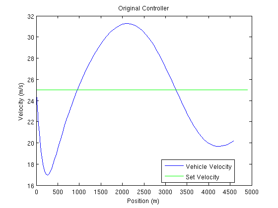
The current controller tuning is inadequate for this road. There are vary large variations in velocity. In order to reduce these variation, the propartional gain K_c was increased by a factor of 5. Below are the results:

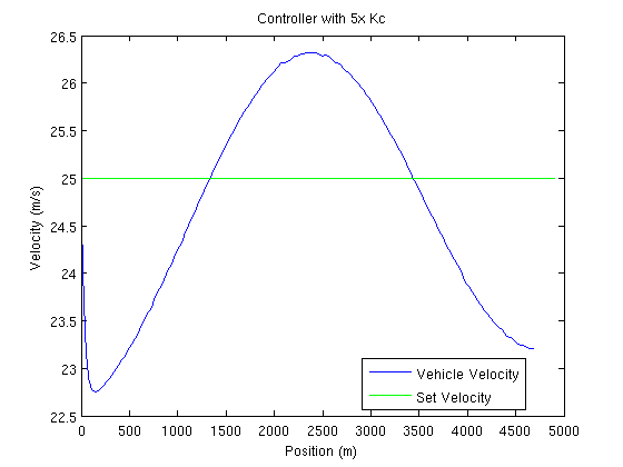
Using the Optimization Toolbox in MATLAB, the controller was optimized by minimizing the sum of the errors (difference between vehicle velocity and set velocity) on this particular segment of road. Below are the optimized controller constants and a plot of the velocity profile:

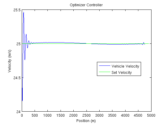
This example shows the power of optimization and model predictive control.

Summary

This example demonstrates the following:

1. Modeling a simple, non-chemical engineering system.
2. Develop a PID controller for said physical dynamical system.
3. Manipulate said system to develop an system of differential equations.
4. Find fixed point(s) for said system.
5. Linearize said system of differential equations.
6. Find the eigenvalues of said linearized system.
7. Construct Root Locus plots for said linearized system.
8. Construct a phase portrait for said dynamical system.
9. Simulate said dynamical system under various conditions.
10. Demonstrate the idea of model predictive control by optimize said controller under a specific scenario.