7.5: Laplace Transforms

Last updated
Save as PDF

Page ID: 22408

$ \newcommand{\vecs}[1]{\overset { \scriptstyle \rightharpoonup} {\mathbf{#1}} } $ $ \newcommand{\vecd}[1]{\overset{-\!-\!\rightharpoonup}{\vphantom{a}\smash {#1}}} $$\newcommand{\id}{\mathrm{id}}$ $ \newcommand{\Span}{\mathrm{span}}$ $ \newcommand{\kernel}{\mathrm{null}\,}$ $ \newcommand{\range}{\mathrm{range}\,}$ $ \newcommand{\RealPart}{\mathrm{Re}}$ $ \newcommand{\ImaginaryPart}{\mathrm{Im}}$ $ \newcommand{\Argument}{\mathrm{Arg}}$ $ \newcommand{\norm}[1]{\| #1 \|}$ $ \newcommand{\inner}[2]{\langle #1, #2 \rangle}$ $ \newcommand{\Span}{\mathrm{span}}$ $\newcommand{\id}{\mathrm{id}}$ $ \newcommand{\Span}{\mathrm{span}}$ $ \newcommand{\kernel}{\mathrm{null}\,}$ $ \newcommand{\range}{\mathrm{range}\,}$ $ \newcommand{\RealPart}{\mathrm{Re}}$ $ \newcommand{\ImaginaryPart}{\mathrm{Im}}$ $ \newcommand{\Argument}{\mathrm{Arg}}$ $ \newcommand{\norm}[1]{\| #1 \|}$ $ \newcommand{\inner}[2]{\langle #1, #2 \rangle}$ $ \newcommand{\Span}{\mathrm{span}}$$\newcommand{\AA}{\unicode[.8,0]{x212B}}$

Introduction

Laplace Transform are frequently used in determining solutions of a wide class of partial diffferential equations. Like other transforms, Laplace transforms are used to determine particular solutions. In solving partial differential equations, the general solutions are difficult, if not impossible, to obtain. Thus, the transform techniques sometimes offer a useful tool for attaining particular solutions. The Laplace transform is closely related to the complex Fourier transform, so the Fourier integral formula can be used to define the Laplace transform and its inverse[3]. Integral transforms are one of many tools that are very useful for solving linear differential equations[1]. An integral transform is a relation of the form:

\[F(s)=\int_{a}^{b} K(s, t) f(t) d t \nonumber \]

where $K(s, t)$ is the kernel of the transformation

The relation given above transforms the function f into another function F, which is called the transform of f. The general idea in using an integral transform to solve a differential equation is as follows:

Use the relation to transform a problem for an unknown function f into a simpler problem for F
Solve this simpler problem to find F
Recover the desired function f from its transform F

Several integral transforms are known to be useful in applied mathematics, but in this chapter we consider only the Laplace transform. This transform is defined in the following way Let f(t) be given for $\leq 0$ . Then the Laplace transform of f, which we will denote by $mathcal{L} \left\{f(t)\right\}$ , is defined by the equation:

\[\mathcal{L}\{f(t)\}=\int_{0}^{\infty} e^{-s t} f(t) d t \nonumber \]

Whenever this improper integral converges. The Laplace transform makes use of the kernel K(s,t) = e⁻(st). Since the solutions of linear differential equations with constant coefficients are bsed on teh exponential function, the Laplace transform is particularly useful for such equations.

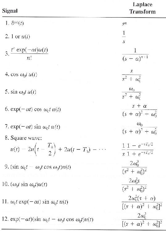
Table 1 - Table of Laplace Transforms

able 5 3 Single sided Laplace Transforms.jpg

Example Problems

Elementary Functions Using Laplace Transforms

Example 1. Given $(c)=c\,\!$ , $\,\!$ is a constant

\[\\mathcal{L}[c] =\int_0^{\infty}e^{-st} c\,dt \,\! \nonumber \]

$=\left [ {-\frac{c e^{-st}}{s}} \right ]_{0}^{\infty}$

$= \frac{c}{s}$

Example 2. Given $f(c)=e^{at}\,\!$ , $a\,\!$ is a constant

\[\\mathcal{L}[e^{at}]=\int_0^{\infty}e^{-st} e^{at}\,dt\,\! \nonumber \]

$=\left [ {-\frac{e^{-(s-a) t}}{(s-a)}} \right ]_{0}^{\infty}$

$=\frac{1}{s-a}$ , where $s \ge a \,\!$

Example 3. Given $f(t)=t^{2} \,\!$ , Then

\[\mathcal{L}\left[t^{2}\right]=\int_{0}^{\infty} e^{-s t} t^{2} d t \nonumber \]

Integration by parts yields

\[=\left[-\frac{t^{2} e^{-s t}}{s}\right]_{0}^{\infty}+\int_{0}^{\infty} \frac{e^{-s t}}{s} 2 t d t \nonumber \]

Since $t^{2} e^{-st} \to 0 \,\!$ as $t \to {\infty} \,\!$ , we have

\[\\mathcal{L}[t^{2}]={\frac{2}{s}} \left [ {-\frac{e^{-st}}{s}}t \right ]_{0}^{\infty}+{\frac{2}{s}} \int_0^{\infty} {\frac{e^{-st}}{s}} \,dt \,\! \nonumber \]

\[ \begin{align*} \mathcal{L}\left[t^{2}\right]=\frac{2}{s}\left[-\frac{e^{-s t}}{s} t\right]_{0}^{\infty}+\frac{2}{s} \int_{0}^{\infty} \frac{e^{-s t}}{s} d t \\[4pt] &= \frac{2}{s^{3}} \end{align*} \nonumber \]

Example 4. Given $f(t) = \sin \omega t \,\!$ . Then

\[F(s)=\mathcal{L}[\sin \omega t]=\int_{0}^{\infty} e^{-s t} \sin \omega t d t \nonumber \]

$= \left [ -{\frac{e^{-st}}{s}} \sin \omega t \right ]_{0}^{\infty} + \int_0^{\infty} {\frac{e^{-st}}{s}} \omega \cos \omega t \,dt \,\!$

$= {\frac{\omega}{s}} \left [ -{\frac{e^{-st}}{s}} \cos \omega t \right ]_{0}^{\infty} - {\frac{\omega}{s}} \int_0^{\infty} {\frac{e^{-st}}{s}} \omega \sin \omega t \,dt \,\!$

$F(s)={\frac{\omega}{s}} - {\frac{\omega^{2}}{s^{2}}} F(s)\,\!$

Thus, solving for $F(s)$, we obtain

\[\mathcal{L}[\sin \omega t]=\frac{\omega}{\left(s^{2}+\omega^{2}\right)} \nonumber \]

In Class Example Using Laplace Transforms

Solving a differential equation:

\[\frac{d y(t)}{d t}=-a y(t) \nonumber \]

Rearranging the equation to one side, we have:

\[\frac{d y(t)}{d t}+a y(t)=0 \nonumber \]

Next, we take the Laplace transform

\[\left(s y(s)-y_{o}\right)+a y(s)=0 \nonumber \]

where $(s) = L[y(t)] \,\!$ and $y_o=y(0) \,\!$ Solving for y(s), we find:

\[y(s)=\frac{y_{o}}{s+a} \nonumber \]

\[y(t)=\mathcal{L}^{-1}\{y(s)\}=\mathcal{L}^{-1}\left\{\frac{y_{o}}{s+a}\right\}=y_{o} e^{-a t} \nonumber \]

References

William E. Boyce, Elementary Differential Equations and Boundary Value Problems (2005) Chapter 6 pp 307-440.
Dr. Ali Muqaibel, EE207 Signals & Systems (2009) <tinyurl.com/ycq46qn>
Tyn Myint-U, Partial Differential Equations for Scientists and Engineers (2005) pp 337 -341.

Contributors and Attributions

Written By: Paul Rhee, Eric Chuang, and David Mui