9.3: PID Tuning via Classical Methods

Introduction

Currently, more than half of the controllers used in industry are PID controllers. In the past, many of these controllers were analog; however, many of today's controllers use digital signals and computers. When a mathematical model of a system is available, the parameters of the controller can be explicitly determined. However, when a mathematical model is unavailable, the parameters must be determined experimentally. Controller tuning is the process of determining the controller parameters which produce the desired output. Controller tuning allows for optimization of a process and minimizes the error between the variable of the process and its set point.

Types of controller tuning methods include the trial and error method, and process reaction curve methods. The most common classical controller tuning methods are the Ziegler-Nichols and Cohen-Coon methods. These methods are often used when the mathematical model of the system is not available. The Ziegler-Nichols method can be used for both closed and open loop systems, while Cohen-Coon is typically used for open loop systems. A closed-loop control system is a system which uses feedback control. In an open-loop system, the output is not compared to the input.

The equation below shows the PID algorithm as discussed in the previous PID Control section.

\[u(t)=K_{c}\left(\epsilon(t)+\frac{1}{\tau_{i}} \int_{0}^{t} \epsilon\left(t^{\prime}\right) d t^{\prime}+\tau_{d} \frac{d \epsilon(t)}{d t}\right)+b \nonumber \]

where

• u is the control signal
• ε is the difference between the current value and the set point.
• K_c is the gain for a proportional controller.
• τ_i is the parameter that scales the integral controller.
• τ_d is the parameter that scales the derivative controller.
• t is the time taken for error measurement.
• b is the set point value of the signal, also known as bias or offset.

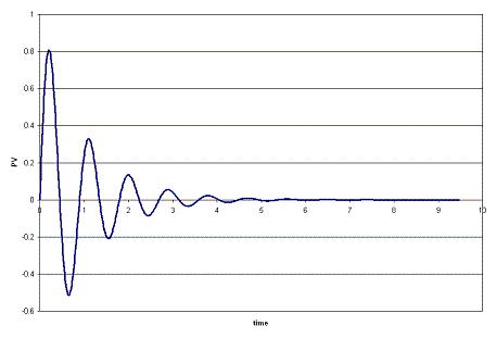
The experimentally obtained controller gain which gives stable and consistent oscillations for closed loop systems, or the ultimate gain, is defined as K_u . K_c is the controller gain which has been corrected by the Ziegler-Nichols or Cohen-Coon methods, and can be input into the above equation. K_u is found experimentally by starting from a small value of K_c and adjusting upwards until consistent oscillations are obtained, as shown below. If the gain is too low, the output signal will be damped and attain equilibrium eventually after the disturbance occurs as shown below.

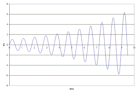
On the other hand, if the gain is too high, the oscillations become unstable and grow larger and larger with time as shown below.

The process reaction curve method section shows the parameters required for open loop system calculations. The Ziegler-Nichols Method section shows how to find K_c, T_i, and T_d for open and closed loop systems, and the Cohen-Coon section shows an alternative way to find K_c, T_i, and T_d.


Open loop systems typically use the quarter decay ratio (QDR) for oscillation dampening. This means that the ratio of the amplitudes of the first overshoot to the second overshoot is 4:1.

Trial and Error

The trial and error tuning method is based on guess-and-check. In this method, the proportional action is the main control, while the integral and derivative actions refine it. The controller gain, K_c, is adjusted with the integral and derivative actions held at a minimum, until a desired output is obtained.

Below are some common values of K_c, T_i, and T_d used in controlling flow, levels, pressure or temperature for trial and error calculations.

Flow

P or PI control can be used with low controller gain. Use PI control for more accuracy with high integration activity. Derivative control is not considered due to the rapid fluctuations in flow dynamics with lots of noise.

K_c = 0.4-0.65

T_i = 6s

Level

P or PI control can be used, although PI control is more common due to inaccuracies incurred due to offsets in P-only control. Derivative control is not considered due to the rapid fluctuations in flow dynamics with lots of noise.

The following P only setting is such that the control valve is fully open when the vessel is 75% full and fully closed when 25% full, being half open when 50% filled.

K_c = 2

Bias b = 50%

Set point = 50%

For PI control:

K_c = 2-20

T_i = 1-5 min

Pressure

Tuning here has a large range of possible values of K_c and T_i for use in PI control, depending on if the pressure measurement is in liquid or gas phase.

Liquid
K_c = 0.5-2

T_i = 6-15 s

Gas
K_c = 2-10

T_i = 2-10 min

Temperature

Due to the relatively slow response of temperature sensors to dynamic temperature changes, PID controllers are used.

K_c = 2-10

T_i = 2-10 min

T_d = 0-5 min

Process Reaction Curve

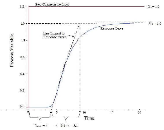
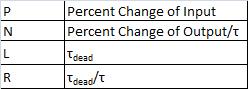
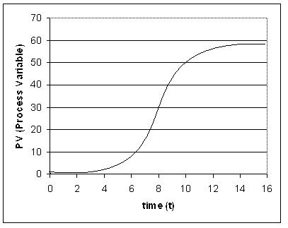
In this method, the variables being measured are those of a system that is already in place. A disturbance is introduced into the system and data can then be obtained from this curve. First the system is allowed to reach steady state, and then a disturbance, X_o, is introduced to it. The percentage of disturbance to the system can be introduced by a change in either the set point or process variable. For example, if you have a thermometer in which you can only turn it up or down by 10 degrees, then raising the temperature by 1 degree would be a 10% disturbance to the system. These types of curves are obtained in open loop systems when there is no control of the system, allowing the disturbance to be recorded. The process reaction curve method usually produces a response to a step function change for which several parameters may be measured which include: transportation lag or dead time, τ_dead, the time for the response to change, τ, and the ultimate value that the response reaches at steady-state, M_u.

τ_dead = transportation lag or dead time: the time taken from the moment the disturbance was introduced to the first sign of change in the output signal

τ = the time for the response to occur

X_o = the size of the step change

M_u = the value that the response goes to as the system returns to steady-state

\[R=\frac{\tau_{\text {dead}}}{\tau} \nonumber \]

\[K_{o}=\frac{X_{o}}{M_{u}} \frac{\tau}{\tau_{\text {dead}}} \nonumber \]

An example for determining these parameters for a typical process response curve to a step change is shown below.
In order to find the values for τ_dead and τ, a line is drawn at the point of inflection that is tangent to the response curve and then these values are found from the graph.

To map these parameters to P,I, and D control constants, see Table 2 and 3 below in the Z-N and Cohen Coon sections.

Ziegler-Nichols Method

In the 1940's, Ziegler and Nichols devised two empirical methods for obtaining controller parameters. Their methods were used for non-first order plus dead time situations, and involved intense manual calculations. With improved optimization software, most manual methods such as these are no longer used. However, even with computer aids, the following two methods are still employed today, and are considered among the most common:

Ziegler-Nichols closed-loop tuning method

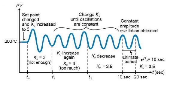
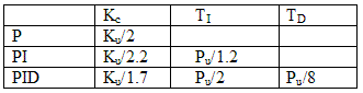
The Ziegler-Nichols closed-loop tuning method allows you to use the ultimate gain value, K_u, and the ultimate period of oscillation, P_u, to calculate K_c . It is a simple method of tuning PID controllers and can be refined to give better approximations of the controller. You can obtain the controller constants K_c , T_i , and T_d in a system with feedback. The Ziegler-Nichols closed-loop tuning method is limited to tuning processes that cannot run in an open-loop environment.

Determining the ultimate gain value, K_u, is accomplished by finding the value of the proportional-only gain that causes the control loop to oscillate indefinitely at steady state. This means that the gains from the I and D controller are set to zero so that the influence of P can be determined. It tests the robustness of the K_c value so that it is optimized for the controller. Another important value associated with this proportional-only control tuning method is the ultimate period (P_u). The ultimate period is the time required to complete one full oscillation while the system is at steady state. These two parameters, K_u and P_u, are used to find the loop-tuning constants of the controller (P, PI, or PID). To find the values of these parameters, and to calculate the tuning constants, use the following procedure:

Closed Loop (Feedback Loop)

1. Remove integral and derivative action. Set integral time (T_i) to 999 or its largest value and set the derivative controller (T_d) to zero.
2. Create a small disturbance in the loop by changing the set point. Adjust the proportional, increasing and/or decreasing, the gain until the oscillations have constant amplitude.
3. Record the gain value (K_u) and period of oscillation (P_u).

Figure 1. System tuned using the Ziegler-Nichols closed-loop tuning method

4. Plug these values into the Ziegler-Nichols closed loop equations and determine the necessary settings for the controller.

Table 1. Closed-Loop Calculations of K_c, T_i, T_d

Advantages

1. Easy experiment; only need to change the P controller
2. Includes dynamics of whole process, which gives a more accurate picture of how the system is behaving

Disadvantages

1. Experiment can be time consuming
2. Can venture into unstable regions while testing the P controller, which could cause the system to become out of control

Ziegler-Nichols Open-Loop Tuning Method or Process Reaction Method:

This method remains a popular technique for tuning controllers that use proportional, integral, and derivative actions. The Ziegler-Nichols open-loop method is also referred to as a process reaction method, because it tests the open-loop reaction of the process to a change in the control variable output. This basic test requires that the response of the system be recorded, preferably by a plotter or computer. Once certain process response values are found, they can be plugged into the Ziegler-Nichols equation with specific multiplier constants for the gains of a controller with either P, PI, or PID actions.

Open Loop (Feed Forward Loop)

To use the Ziegler-Nichols open-loop tuning method, you must perform the following steps:

1. Make an open loop step test

2. From the process reaction curve determine the transportation lag or dead time, τ_dead, the time constant or time for the response to change, τ, and the ultimate value that the response reaches at steady-state, M_u, for a step change of Xo.

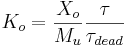
3. Determine the loop tuning constants. Plug in the reaction rate and lag time values to the Ziegler-Nichols open-loop tuning equations for the appropriate controller—P, PI, or PID—to calculate the controller constants. Use the table below.

Table 2. Open-Loop Calculations of K_c, T_i, T_d

Advantages

1. Quick and easier to use than other methods
2. It is a robust and popular method
3. Of these two techniques, the Process Reaction Method is the easiest and least disruptive to implement

Disadvantages

1. It depends upon purely proportional measurement to estimate I and D controllers.
2. Approximations for the K_c, T_i, and T_d values might not be entirely accurate for different systems.
3. It does not hold for I, D and PD controllers

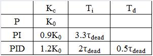
Cohen-Coon Method

The Cohen-Coon method of controller tuning corrects the slow, steady-state response given by the Ziegler-Nichols method when there is a large dead time (process delay) relative to the open loop time constant; a large process delay is necessary to make this method practical because otherwise unreasonably large controller gains will be predicted. This method is only used for first-order models with time delay, due to the fact that the controller does not instantaneously respond to the disturbance (the step disturbance is progressive instead of instantaneous).

The Cohen-Coon method is classified as an 'offline' method for tuning, meaning that a step change can be introduced to the input once it is at steady-state. Then the output can be measured based on the time constant and the time delay and this response can be used to evaluate the initial control parameters.

For the Cohen-Coon method, there are a set of pre-determined settings to get minimum offset and standard decay ratio of 1/4(QDR). A 1/4(QDR) decay ratio refers to a response that has decreasing oscillations in such a manner that the second oscillation will have 1/4 the amplitude of the first oscillation . These settings are shown in Table 3..

Table 3. Standard recommended equations to optimize Cohen Coon predictions

where the variables P, N, and L are defined below.

Alternatively, K₀ can be used instead of (P/NL). K₀,τ, and τ_dead are defined in process reaction curve section. An example using these parameters is shown here [1].

The process in Cohen-Coon turning method is the following:

1. Wait until the process reaches steady state.
2. Introduce a step change in the input.
3. Based on the output, obtain an approximate first order process with a time constant τ delayed by τ_dead units from when the input step was introduced.

The values of τ and τ_dead can be obtained by first recording the following time instances:

t0 = time at input step start point t2 = time when reaches half point t3 = time when reaches 63.2% point

4. Using the measurements at t0, t2, t3, A and B, evaluate the process parameters τ, τ_dead, and K_o.

5. Find the controller parameters based on τ, τ_dead, and K_o.

Advantages

1. Used for systems with time delay.
2. Quicker closed loop response time.

Disadvantages and Limitations

1. Unstable closed loop systems.
2. Can only be used for first order models including large process delays.
3. Offline method.
4. Approximations for the K_c, τ_i, and τ_d values might not be entirely accurate for different systems.

Other Methods

These are other common methods that are used, but they can be complicated and aren't considered classical methods, so they are only briefly discussed.

Internal Model Control

The Internal Model Control (IMC) method was developed with robustness in mind. The Ziegler-Nichols open loop and Cohen-Coon methods give large controller gain and short integral time, which isn't conducive to chemical engineering applications. The IMC method relates to closed-loop control and doesn't have overshooting or oscillatory behavior. The IMC methods however are very complicated for systems with first order dead time.

Auto Tune Variation

The auto-tune variation (ATV) technique is also a closed loop method and it is used to determine two important system constants (P_u and K_u for example). These values can be determined without disturbing the system and tuning values for PID are obtained from these. The ATV method will only work on systems that have significant dead time or the ultimate period, P_u, will be equal to the sampling period.

Example \(\PageIndex{1}\)

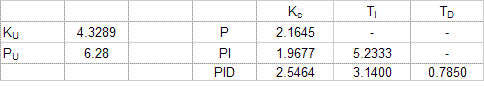
You're a controls engineer working for Flawless Design company when your optimal controller breaks down. As a backup, you figure that by using coarse knowledge of a classical method, you may be able to sustain development of the product. After adjusting the gain to one set of data taken from a controller, you find that your ultimate gain is 4.3289.

From the adjusted plot below, determine the type of loop this graph represents; then, please calculate K_c, T_i, and T_d for all three types of controllers.

Solution

From the fact that this graph oscillates and is not a step function, we see that this is a closed loop. Thus, the values will be calculated accordingly.

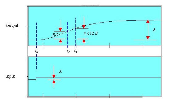
We're given the Ultimate gain, K_u = 4.3289. From the graph below, we see that the ultimate period at this gain is P_u = 6.28

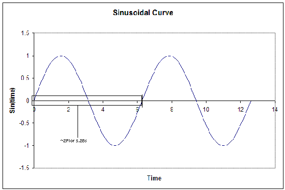
From this, we can calculate the K_c, T_i, and T_d for all three types of controllers. The results are tabulated below. (Results were calculated from the Ziegler-Nichols closed-loop equations.)

Example \(\PageIndex{2}\)

Your partner finds another set of data after the controller breaks down and decides to use the Cohen-Coon method because of the slow response time for the system. They also noticed that the control dial, which goes from 0-8, was set at 3 instead of 1. Luckily the response curve was obtained earlier and is illustrated below. From this data he wanted to calculate K_c, T_i and T_d. Help him to determine these values. Note that the y-axis is percent change in the process variable.

Solution

In order to solve for K_c, T_i and T_d, you must first determine L, ΔC_p, and T. All of these values may be calculated by the reaction curve given.

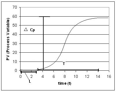
From the process reaction curve we can find that:
\(L = 3\)
\(T = 11\)
\(ΔC__p = 0.55\, (55%)\)

Now that these three values have been found N and R may be calculated using the equations below.

N =
R =

Using these equations you find that
N = .05
R = 0.27
We also know that since the controller was moved from 1 to 3, so a 200% change.
P = 2.00

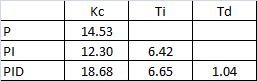
We use these values to calculate K_c, T_i, and T_d, for the three types of controllers based on the equations found in Table 3.

Tuning the parameters of a PID controller on an actual system

There are several ways to tune the parameters of a PID controller. They involve the following procedures. For each, name the procedure and explain how the given measured information is used to pick the parameters of the PID controller.

Example \(\PageIndex{1}\)

1. The controller is set to P only, and the system is operated in "closed-loop", meaning that the controller is connected and working. The gain is tuned up until a resonance is obtained. The amplitude and frequency of that resonance is measured.
2. The system is kept in "open-loop" mode, and a step-function change is manually made to the system (through a disturbance or through the controller itself). The resulting response of the system is recorded as a function of time.

Solution

a. We will use the Ziegler-Nichols method.

Ki=0.5Ku
Ku is the ultimate gain when the system started oscillating.

b. We will use the Cohen-Coon method.

We can locate the inflection point of the step function and draw a tangent. Τ_dead is located at the crossing of that tangent with t, and Τ is located at the cross of the tangent with M(t)

Exercise \(\PageIndex{1}\)

Which of the following do you RECORD during the Ziegler-Nichols Method?

1. \(K_c\)
2. \(τ_i\)
3. \(K_o\)
4. \(τ_d\)

Answer

Answer:C

Exercise \(\PageIndex{2}\)

For the Ziegler-Nichols Method, it is important to:

1. Find a gain that produces damped oscillation
2. Set P and I controllers to zero
3. Record the period of oscillation
4. Calculate T_c

Answer

Answer:A,C

References

• Svrcek, William Y., Mahoney, Donald P., Young, Brent R. A Real Time Approach to Process Control, 2nd Edition. John Wiley & Sons, Ltd.
• Astrom, Karl J., Hagglund, Tore., Advanced PID Control, ISA, The Instrumentation, Systems and Automation Society.
• "ACT Ziegler-Nichols Tuning," ourworld.compuserve.com/homepages/ACTGMBH/zn.htm
• Ogata, Katsuhiko. System Dynamics, 4th Edition. Pearson Education, Inc.