11.4: Ratio Control

Introduction

Ratio control architecture is used to maintain the relationship between two variables to control a third variable. Perhaps a more direct description in the context of this class is this: Ratio control architecture is used to maintain the flow rate of one (dependent controlled feed) stream in a process at a defined or specified proportion relative to that of another (independent wild feed stream) (3) in order to control the composition of a resultant mixture.

As hinted in the definition above, ratio control architectures are most commonly used to combine two feed streams to produce a mixed flow of a desired composition or physical property downstream (3). Ratio controllers can also control more than two streams. Theoretically, an infinite number of streams can be controlled by the ratio controller, as long as there is one controlled feed stream. In this way, the ratio control architecture is feedfoward in nature. In this context, the ratio control architecture involves the use of an independent wild feed stream and a dependent stream called the controlled feed.

Ratio Control is the most elementary form of feed forward control. These control systems are almost exclusively applied to flow rate controls. There are many common usages of ratio controls in the context of chemical engineering. They are frequently used to control the flows on chemical reactors. In these cases, they keep the ratio of reactants entering a reaction vessel in correct proportions in order to keep the reaction conditions ideal. They are also frequently used for large scale dilutions.

Ratio Control based upon Error of a Variable Ratio

The first type of ratio control architecture uses the error of a variable ratio (\(R_{actual}\)) from a set ratio (\(R_{set}\)) to manipulate y (the controlled stream). \(R_{actual}\) is a ratio of the two variables wild stream and controlled stream. The controller adjusts the flow rate of stream \(y\) (controlled stream) in a manner appropriate for the error (\(R_{actual} - R_{set}\)).

The error in this system would be represented using the following equations:

\[\frac{y}{y_{w}}=R_{\text {actual }} \nonumber \]

or

\[\frac{y_{w}}{y}=R_{\text {actual }} \nonumber \]

with

\[\text{Error} =R_{\text {actual }}-R_{\text {set }} \nonumber \]

This error would be input to your general equation for your P, PI, or PID controller as shown below.

\[V_{y}=Offset +K_{c}(Error)+\frac{1}{\tau_{I}} \int(\text {Error}) d t+\tau_{D} \frac{d(\text {Error})}{d t} \nonumber \]

NOTE: Vy is used instead of y, because y is not directly adjustable. The only way to adjust y is to adjust the valve (V) that affects y.

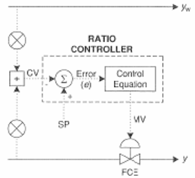
4.2.1 Diagram of Ratio Dependant System. Image taken from Svreck et al.

Ratio Control based upon Error of the Controlled Stream

The second type of ratio control architecture uses the error of a setpoint (yset, setpoint of the control variable) from y (controlled variable) to control, once again, y. The controller adjusts the flow rate of stream y in a manner appropriate for the error (y-yset).

The error in this system would be represented using the following equation:

\[\boldsymbol{y}_{w} \boldsymbol{R}_{s e t}=\boldsymbol{y}_{s e t} \nonumber \]

or

\[\frac{\boldsymbol{y}_{w}}{\boldsymbol{R}_{\text {set}}}=\boldsymbol{y}_{\text {set}} \nonumber \]

with

\[\text{Error} =y-y_{\text {set }} \nonumber \]

This error would be input to your general equation for your P, PI, or PID controller as shown below.

\[V_{y}= \text{Offset} + K_{c}(Error)+\frac{1}{\tau_{I}} \int(Error) d t+\tau_{D} \frac{d(Error)}{d t} \nonumber \]

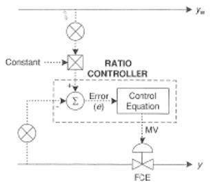
4.3.1 Diagram of Flowrate Dependant System. Image taken from Svreck et al.

Comparing the Two Types of Ratio Control

The main difference between the two aforementioned types of ratio control architecture is that they respond to changes in the monitored variable (Ractual or y - the variables through which the error is determined) differently.

The first method mentioned that defines error as (R_{actual}-R_{set}\) (monitored variable of \(R_{actual}\)) responds sluggishly when y is relatively large and too quickly when y is relatively small. This is best explained by examining the equations below.

\[\begin{align}
R&=\frac{y_{w}}{y} \longrightarrow \frac{\partial(R)}{\partial\left(y_{w}\right)}=\frac{1}{y} \\
R&=\frac{y}{y_{w}} \longrightarrow \frac{\partial(R)}{\partial\left(y_{w}\right)}=-\frac{y}{y_{w}^{2}}
\end{align} \nonumber \]

Unlike the first method, the second method mentioned that defines error as \(y-y_{set}\) (monitored variable of y) does not respond differently depending upon the relative amounts of y (or anything else, for that matter). This is best explained by examining the equations below.

\[\begin{align}
y&=y_{w} R_{y t t} \longrightarrow \frac{\partial(y)}{\partial\left(y_{w}\right)}=R_{y t t} \\
y&=\frac{y_{w}}{R_{s e t}} \longrightarrow \frac{\partial(y)}{\partial\left(y_{w}\right)}=\frac{1}{R_{y e t}}
\end{align} \nonumber \]

Difficulties with Ratio Controllers

Steady State Issues

A common difficulty encountered with ratio controllers occurs when the system is not at steady state. Unsteady state conditions can cause a delay in the adjustment of the manipulated flow rate and thus the desired state of the system cannot be met.

Blend Stations

To overcome the difficulty with steady state, a Blend station can be used, which takes into account both the set ratio and the wild stream. As can be seen by the diagram below, the Blend station takes in the wild stream flow rate, the set ratio, and the initial set point for the wild stream (r1) as inputs. Using a weighting factor, called gain, the Blend station determines a new set point for the manipulated stream (r2). The relationship that determines this new set point can be seen below.

\[r_{2}=\operatorname{set} r a t i o\left[\gamma^{*} r_{1}+(1-\gamma) y_{w}\right] \nonumber \]

where \(γ\) is the gain factor.

Image taken from Astrom and Hagglund article on "Advanced PID Control."

Accuracy Issues

Another problem (which is an issue with all "feed-forward" controllers) is that the variable under control (mix ratio) is not directly measured. This requires a highly accurate characterization of the controlled stream's valves so that the desired flow rate is actually matched.

One way to address this problem is to use two levels of PID control (Cascade Control). The first level monitors the controlled streams flow rate and adjusts it to the desired set point with a valve. The outer level of control monitors the wild stream’s flow rate which adjusts the set point of the controlled stream by multiplying by the desired ratio. For example, if stream A’s flow rate is measured as 7 gpm, and the desired ratio of A:B is 2, then the outer level of control will adjust B’s set point to 3.5. Then the inner level of control will monitor B’s flow rate until it achieves a flow rate of 3.5.

Ratio Control Schemes

The following subsections introduce three ratio controller schematics. Each schematic illustrates different ways that the controlled feed stream can be manipulated to account for the varying wild feed stream.

Ratio Relay Controller

The wild feed flow rate is received by the ratio relay and then multiplied by the desired mix ratio. The ratio relay outputs the calculated controlled feed flow rate which is compared to the actually flow rate of the controlled feed stream. The flow controller then adjusts the controlled feed flow rate so that it matches the set point (3).

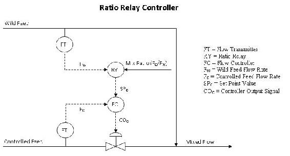
Image adapted from Houtz, Allen and Cooper, Doug "The Ratio Control Architecture"

The mix ratio (Fc/Fw) is not easy to access, so it requires a high level of authorization to change. This higher level of security may be an advantage so that only permitted people can change the mix ratio and decrease the chance that an accidental error occurs. A disadvantage is that if the mix ratio does need to be changed quickly, operation may be shut down while waiting for the appropriate person to change it.

Another disadvantage is that linear flow signals are required. The output signals from the flow transmitters, Fw and Fc, must change linearly with a change in flow rate. Turbine flow meters provide signals that change linearly with flow rates. However, some flow meters like orifice meters require additional computations to achieve a linear relationship between the flow rate and signal.

Flow Fraction Controller

Flow fraction and ratio relay controllers are very similar except that the flow fraction controller has the advantage of being a single-input single-output controller. A flow fraction controller receives the wild feed and controlled feed flow rates directly. The desired ratio of the controlled feed to wild feed is a preconfigured option in modern computer control systems (3).

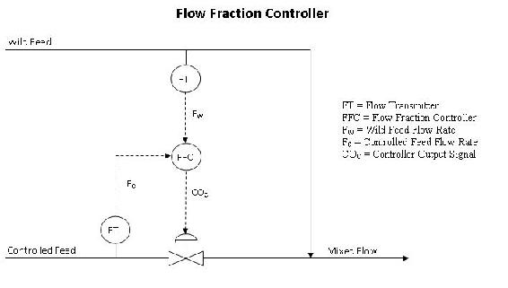
Image adapted from Houtz, Allen and Cooper, Doug "The Ratio Control Architecture"

Ratio Relay with Remote Input

The ratio relay with remote input model of a ratio controller is similar to the cascade control model in that it is part of a larger control strategy. The purpose of this model is to account for any unexpected or unmeasured changes that have occurred in the wild and controller feed streams. The diagram below illustrates how the composition of the mixed flow is used to change the relay ratio (3).

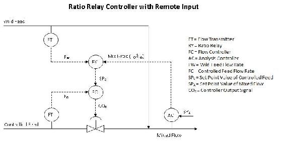
Image adapted from Houtz, Allen and Cooper, Doug "The Ratio Control Architecture"

The main advantage of having remote input is that the mix ratio is constantly being updated. A disadvantage of using an additional analyzer is that the analysis of the mixed stream may take a long time and decrease the control performance. The lag time depends on the type of sensor being used. For example, a pH sensor will most likely returned fast, reliable feedback while a spectrometer would require more time to analyze the sample.

Advantages and Disadvantages

There are some pros and cons to using ratio control where there is a ratio being maintained between two flow rates.

Advantages

1. Allows user to link two streams to produce and maintain a defined ratio between the streams
2. Simple to use
3. Does not require a complex model

Disadvantages

1. Often one of the flow rates is not measured directly and the controller assumes that the flows have the correct ratio through the control of only the measured flow rate
2. Requires a ratio relationship between variables that needs to be maintained
3. Not as useful for variables other than flow rates

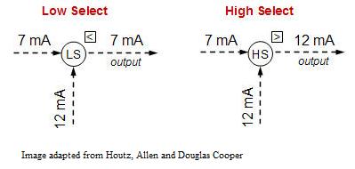
Select Elements in Ratio Control

A select element enables further control sophistication by adding decision-making logic to the ratio control system. By doing so, a select variable can be controlled to a maximum or minimum constraint. The figure below depicts the basic action of both a low select and high select controller.

Single Select Override Control

Often times, these select elements are used as an override element in ratio control. Take, for example, ratio control system (with remote input) of a metered-air combustion process in the figure below.

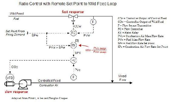
In this design, the fuel set point, SPw, comes in as firing demand from a different part of the plant, so fuel flow rate cannot be adjusted freely. As the fuel set point (and therefore fuel mass flow rate, PVw) fluctuates, a ratio relay is employed to compute the combustion air set point, SPc. If the flow command outputs (COw and COc) are able to respond quickly, then the system architecture should maintain the desired air/fuel ratio despite the demand set point varying rapidly and often. However, sometimes the final control element (such as the valve on the fuel feed stream and blower on the combustion air feed stream in the diagram) can have a slow response time. Ideally, the flow rates would fluctuate in unison to maintain a desired ratio, but the presence of a slow final control element may not allow the feed streams to be matched at that desired ratio for a significant period of time. Valves often have quick response times, however, blowers like the one controlling the combustion air feed stream can have slow response times. A solution to this problem is to add a “low select” override to the control system, as shown in the figure below.

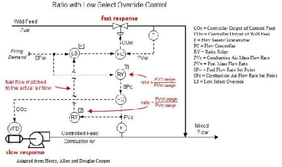
The second ratio controller will receive the actual measured combustion air mass flow rate and compute a matching fuel flow rate based on the ideal design air/fuel mixture. This value is then transmitted to the low select controller, which also receives fuel flow rate set point based from the firing demand. The low select controller then has the power to pass the lower of the two input signals forward. So, if the fuel flow rate firing demand exceeds combustion air availability required to burn the fuel, then the low select controller can override the firing demand and pass along the signal of the fuel flow rate calculated based on the actual air flow (from the second ratio relay).

This low select override strategy ensures that the proper air/fuel ratio will be maintained when the firing demand rapidly increases, but does not have an effect when the firing demand is rapidly decreasing. While the low select override can help eliminate pollution when firing demand rates increase quickly, a rapid decrease in firing demand can cause incomplete combustion (as well as increased temperature) and loss of profit.

Cross-Limiting Override Control

Cross-limiting override control utilizes the benefit of multiple select controls. Most commonly, a control system using the cross-limiting override strategy will implement both a high select and low select control. As a result, the system can account for quickly increasing firing demand as well as quickly decreasing firing demand. The figure below depicts a such a scenario using the inlet combustion air and fuel for a boiler as the example.

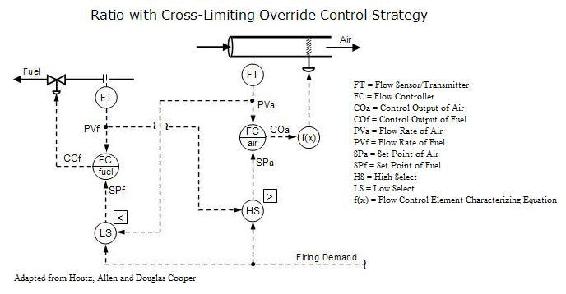
It is assumed that same firing demand enters the high select and low select control and the flow transmitters have been calibrated so that the ideal air/fuel ratio is achieved when both signal match. As a result, the set point of air will always be the greater value of the firing demand and current fuel flow signals. Likewise, the set point of fuel will always be the lower value of the firing demand and current air flow signals. So, as the firing demand increases, the set point of air will increase. At the same time, the low select will keep the set point of fuel to the signal set by the present flow or air. Therefore, the set point of fuel will not match the increasing firing demand, but will follow the increasing air flow rate as it is responding upwards. Similarly, if the firing demand decreases, the low select control will listen to the firing demand and the high select controller will not. As a result, the firing demand will directly cause the set point of fuel to decrease while the set point of air will follow the decreasing fuel rate as it responds downwards. The cross-limiting override strategy allows for greater balance in a ratio control system.

Worked out Example 1

In the following process shown below, a concentrated solution of product is diluted continuously to be sold as a final 10% solution. Flowrates coming from the unit feeding the pure product to this mixing tank are not constant (the wild stream), and therefore a ratio controller is used to properly dilute the solution.

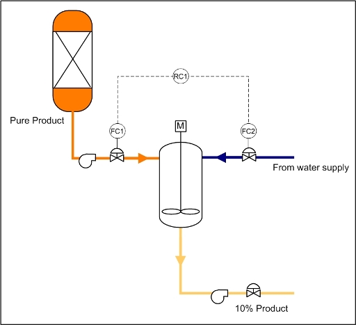
In this example, the ratio controller would be set to a value of FC1/FC2 = RC1 = 9. The ratio contoller in this case would then work by the following logic:

For an additional challenge, determine an error equation that can is related to this controller.

Worked out Example 2

One of the most common uses of a ratio controller is used for correcting the air-fuel ratio in automobiles. A specified amount of air is always taken up by the engine and the amount of fuel injected is controlled by a computer through the use of a ratio controller. The stoichiometric ratio for air to gasoline by mass is 14.7:1. There is an oxygen sensor in the exhaust manifold as well as sensors for all of the exhaust components. This sensor is connected to the valve for the fuel injection. If there is too much oxygen measured in the exhaust, then the mixture is said to be lean. Is the ratio of air to gas in the original mixture greater than or less than 14.7:1 and what should the valve controlling the fuel injection do?

Note: This is an indirect form of a ratio controller as it measuring a physical property of downstream in order to determine if the ratio is too high or low. Further information may be found here about Air-fuel Ratio and Oxygen Sensors.

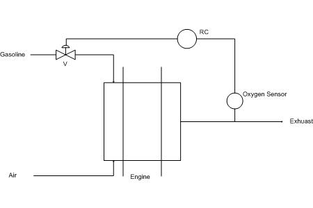
Answer: Since there is leftover oxygen in the exhaust, there must have been too much in the original mixture. The ratio of air to gas in the original mixture is greater than 14.7:1 and thus the computer should open the valve more for the fuel injection.

Worked out Example 3

Many processes in industry require multiple process streams entering at different locations in the system. A senior engineer gives you the project to design the control scheme for a new process to be implemented at the company. The process involves 2 reactions and 3 different feed streams.

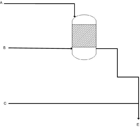
Reactions: 2A + B --> D

\[\ce{C + 3D -> E} \nonumber \]

Assume the reactions go to 100% completion (you only need stoichiometric amounts).

Complete the P&ID with the control scheme and write the ratios (with respect to B) that the other molar flow rates will be set to. Also explain how the system will take action when it detects excess C or D in the product stream.

Solution:

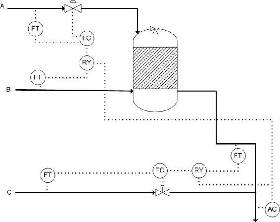
A: 2 B: 1 C: 1 D: 1/3 E: 1/3

If the AC detects greater or less amounts of C expected, it will adjust the ratio setting in RY connected to C's flow controller, reducing or decreasing the ratio of C to B, respectively.

Exercise \(\PageIndex{1}\)

Why is a Blend Station used?

1. to create the set point for the ratio controller
2. to reduce lag time in adjusting flow rates
3. to measure flow rates
4. to multiply one flow rate by the desired ratio

Answer

TBA

Exercise \(\PageIndex{2}\)

How is the set ratio used in the first type of ratio controller described above?

1. Outputs how much each stream should be flowing.
2. It is compared against two flow rates to adjust one if needed.
3. Tells the system to shut down.
4. It adjusts for lag time when the system is not at steady-state.

Answer

Add texts here. Do not delete this text first.

References

• Astrom, Karl J. and Hagglund, Torr. "Advanced PID Control" The Instrumentation, Systems and Automation Society.
• Mahoney, Donald P., Svrcek, William Y. and Young, Brent R. "A Real-Time Approach to Process Control", Second Edition. John Wiley & Sons, Ltd.
• Houtz, Allen and Cooper, Doug "The Ratio Control Architecture" http://www.controlguru.com (http://www.controlguru.com/2007/120207.html)