13.1: Basic statistics- mean, median, average, standard deviation, z-scores, and p-value

Statistics is a field of mathematics that pertains to data analysis. Statistical methods and equations can be applied to a data set in order to analyze and interpret results, explain variations in the data, or predict future data. A few examples of statistical information we can calculate are:

• Average value (mean)
• Most frequently occurring value (mode)
• On average, how much each measurement deviates from the mean (standard deviation of the mean)
• Span of values over which your data set occurs (range), and
• Midpoint between the lowest and highest value of the set (median)

Statistics is important in the field of engineering by it provides tools to analyze collected data. For example, a chemical engineer may wish to analyze temperature measurements from a mixing tank. Statistical methods can be used to determine how reliable and reproducible the temperature measurements are, how much the temperature varies within the data set, what future temperatures of the tank may be, and how confident the engineer can be in the temperature measurements made. This article will cover the basic statistical functions of mean, median, mode, standard deviation of the mean, weighted averages and standard deviations, correlation coefficients, z-scores, and p-values.

What is a Statistic?

In the mind of a statistician, the world consists of populations and samples. An example of a population is all 7th graders in the United States. A related example of a sample would be a group of 7th graders in the United States. In this particular example, a federal health care administrator would like to know the average weight of 7th graders and how that compares to other countries. Unfortunately, it is too expensive to measure the weight of every 7th grader in the United States. Instead statistical methodologies can be used to estimate the average weight of 7th graders in the United States by measure the weights of a sample (or multiple samples) of 7th graders.

Parameters are to populations as statistics are to samples.

A parameter is a property of a population. As illustrated in the example above, most of the time it is infeasible to directly measure a population parameter. Instead a sample must be taken and statistic for the sample is calculated. This statistic can be used to estimate the population parameter. (A branch of statistics know as Inferential Statistics involves using samples to infer information about a populations.) In the example about the population parameter is the average weight of all 7th graders in the United States and the sample statistic is the average weight of a group of 7th graders.

A large number of statistical inference techniques require samples to be a single random sample and independently gathers. In short, this allows statistics to be treated as random variables. A in-depth discussion of these consequences is beyond the scope of this text. It is also important to note that statistics can be flawed due to large variance, bias, inconsistency and other errors that may arise during sampling. Whenever performing over reviewing statistical analysis, a skeptical eye is always valuable.

Statistics take on many forms. Examples of statistics can be seen below.

Basic Statistics

When performing statistical analysis on a set of data, the mean, median, mode, and standard deviation are all helpful values to calculate. The mean, median and mode are all estimates of where the "middle" of a set of data is. These values are useful when creating groups or bins to organize larger sets of data. The standard deviation is the average distance between the actual data and the mean.

Mean and Weighted Average

The mean (also know as average), is obtained by dividing the sum of observed values by the number of observations, n. Although data points fall above, below, or on the mean, it can be considered a good estimate for predicting subsequent data points. The formula for the mean is given below as Equation \ref{1}. The excel syntax for the mean is AVERAGE(starting cell: ending cell).

\[\bar{X}=\frac{\sum_{i=1}^{i=n} X_{i}}{n} \label{1} \]

However, equation (1) can only be used when the error associated with each measurement is the same or unknown. Otherwise, the weighted average, which incorporates the standard deviation, should be calculated using equation (2) below.

\[X_{w a v}=\frac{\sum w_{i} x_{i}}{\sum w_{i}} \label{2} \]

where \[w_{i}=\frac{1}{\sigma_{i}^{2}}\nonumber \] and \(x_i\) is the data value.

Median

The median is the middle value of a set of data containing an odd number of values, or the average of the two middle values of a set of data with an even number of values. The median is especially helpful when separating data into two equal sized bins. The excel syntax to find the median is MEDIAN(starting cell: ending cell).

Mode

The mode of a set of data is the value which occurs most frequently. The excel syntax for the mode is MODE(starting cell: ending cell).

Considerations

Now that we've discussed some different ways in which you can describe a data set, you might be wondering when to use each way. Well, if all the data points are relatively close together, the average gives you a good idea as to what the points are closest to. If on the other hand, almost all the points fall close to one, or a group of close values, but occasionally a value that differs greatly can be seen, then the mode might be more accurate for describing this system, whereas the mean would incorporate the occasional outlying data. The median is useful if you are interested in the range of values your system could be operating in. Half the values should be above and half the values should be below, so you have an idea of where the middle operating point is.

Standard Deviation and Weighted Standard Deviation

The standard deviation gives an idea of how close the entire set of data is to the average value. Data sets with a small standard deviation have tightly grouped, precise data. Data sets with large standard deviations have data spread out over a wide range of values. The formula for standard deviation is given below as Equation \ref{3}. The excel syntax for the standard deviation is STDEV(starting cell: ending cell).

\[\sigma=\sqrt{\frac{1}{n-1} \sum_{i=1}^{i=n}\left(X_{i}-\bar{X}\right)^{2}} \label{3} \]

Side Note: Bias Estimate of Population Variance

The standard deviation (the square root of variance) of a sample can be used to estimate a population's true variance. Equation \ref{3} above is an unbiased estimate of population variance. Equation \ref{3.1} is another common method for calculating sample standard deviation, although it is an bias estimate. Although the estimate is biased, it is advantageous in certain situations because the estimate has a lower variance. (This relates to the bias-variance trade-off for estimators.)

\[\sigma_{n}=\sqrt{\frac{1}{n} \sum_{i=1}^{i=n}\left(X_{i}-\bar{X}\right)^{2}} \label{3.1} \]

When calculated standard deviation values associated with weighted averages, Equation \ref{4} below should be used.

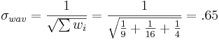
\[\sigma_{w a v}=\frac{1}{\sqrt{\sum w_{i}}} \label{4} \]

The Sampling Distribution and Standard Deviation of the Mean

Population parameters follow all types of distributions, some are normal, others are skewed like the F-distribution and some don't even have defined moments (mean, variance, etc.) like the Chaucy distribution. However, many statistical methodologies, like a z-test (discussed later in this article), are based off of the normal distribution. How does this work? Most sample data are not normally distributed.

This highlights a common misunderstanding of those new to statistical inference. The distribution of the population parameter of interest and the sampling distribution are not the same. Sampling distribution?!? What is that?

Imagine an engineering is estimating the mean weight of widgets produced in a large batch. The engineer measures the weight of N widgets and calculates the mean. So far, one sample has been taken. The engineer then takes another sample, and another and another continues until a very larger number of samples and thus a larger number of mean sample weights (assume the batch of widgets being sampled from is near infinite for simplicity) have been gathered. The engineer has generated a sample distribution.

As the name suggested, a sample distribution is simply a distribution of a particular statistic (calculated for a sample with a set size) for a particular population. In this example, the statistic is mean widget weight and the sample size is N. If the engineer were to plot a histogram of the mean widget weights, he/she would see a bell-shaped distribution. This is because the Central Limit Theorem guarantees that as the sample size approaches infinity, the sampling distributions of statistics calculated from said samples approach the normal distribution.

Conveniently, there is a relationship between sample standard deviation (σ) and the standard deviation of the sampling distribution ( - also know as the standard deviation of the mean or standard error deviation). This relationship is shown in Equation \ref{5} below:

\[\sigma_{\bar{X}}=\frac{\sigma_{X}}{\sqrt{N}} \label{5} \]

An important feature of the standard deviation of the mean, is the factor in the denominator. As sample size increases, the standard deviation of the mean decrease while the standard deviation, σ does not change appreciably.

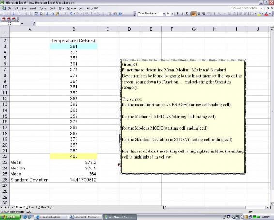
Microsoft Excel has built in functions to analyze a set of data for all of these values. Please see the screen shot below of how a set of data could be analyzed using Excel to retrieve these values.

Example by Hand

You obtain the following data points and want to analyze them using basic statistical methods. {1,2,2,3,5}

Calculate the average: Count the number of data points to obtain \(n = 5\)

\[mean =\frac{1+2+2+3+5}{5}=2.6\nonumber \]

Obtain the mode: Either using the excel syntax of the previous tutorial, or by looking at the data set, one can notice that there are two 2's, and no multiples of other data points, meaning the 2 is the mode.

Obtain the median: Knowing the n=5, the halfway point should be the third (middle) number in a list of the data points listed in ascending or descending order. Seeing as how the numbers are already listed in ascending order, the third number is 2, so the median is 2.

Calculate the standard deviation: Using Equation \ref{3},

\[\sigma =\sqrt{\frac{1}{5-1} \left( 1 - 2.6 \right)^{2} + \left( 2 - 2.6\right)^{2} + \left(2 - 2.6\right)^{2} + \left(3 - 2.6\right)^{2} + \left(5 - 2.6\right)^{2}} =1.52\nonumber \]

Example by Hand (Weighted)

Three University of Michigan students measured the attendance in the same Process Controls class several times. Their three answers were (all in units people):

• Student 1: A = 100 ± 3
• Student 2: A = 105 ± 4
• Student 3: A = 102 ± 2

What is the best estimate for the attendance A?

, , ,

Therefore,

\[A = 101.92 ± 0.65\, students \nonumber \]

Gaussian Distribution

Gaussian distribution, also known as normal distribution, is represented by the following probability density function:

\[P D F_{\mu, \sigma}(x)=\frac{1}{\sigma \sqrt{2 \pi}} e^{-\frac{(x-\mu)^{2}}{2 \sigma^{2}}}\nonumber \]

where μ is the mean and σ is the standard deviation of a very large data set. The Gaussian distribution is a bell-shaped curve, symmetric about the mean value. An example of a Gaussian distribution is shown below.

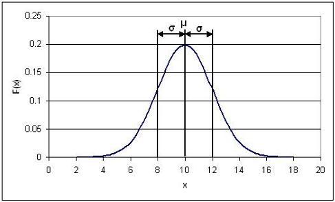
In this specific example, μ = 10 and σ = 2.

Probability density functions represent the spread of data set. Integrating the function from some value x to x + a where a is some real value gives the probability that a value falls within that range. The total integral of the probability density function is 1, since every value will fall within the total range. The shaded area in the image below gives the probability that a value will fall between 8 and 10, and is represented by the expression:

Gaussian distribution is important for statistical quality control, six sigma, and quality engineering in general. For more information see What is 6 sigma?.

Error Function

A normal or Gaussian distribution can also be estimated with a error function as shown in the equation below.

\[P(8 \leq x \leq 10)=\int_{8}^{10} \frac{1}{\sigma \sqrt{2 \pi}} e^{-\frac{(x-\mu)^{2}}{2 \sigma^{2}}} d x=\operatorname{erf}(t)\nonumber \]

Here, erf(t) is called "error function" because of its role in the theory of normal random variable. The graph below shows the probability of a data point falling within t*σ of the mean.

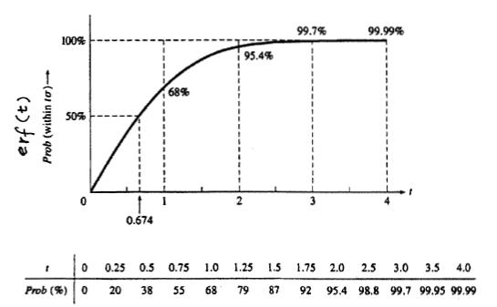
For example if you wanted to know the probability of a point falling within 2 standard deviations of the mean you can easily look at this table and find that it is 95.4%. This table is very useful to quickly look up what probability a value will fall into x standard deviations of the mean.

Correlation Coefficient (r value)

The linear correlation coefficient is a test that can be used to see if there is a linear relationship between two variables. For example, it is useful if a linear equation is compared to experimental points. The following equation is used:

\[r=\frac{\sum\left(X_{i}-X_{\text {mean}}\right)\left(Y_{i}-Y_{\text {mean}}\right)}{\sqrt{\sum\left(X_{i}-X_{\text {mean}}\right)^{2}} \sqrt{\sum\left(Y_{i}-Y_{\text {mean}}\right)^{2}}}\nonumber \]

The range of r is from -1 to 1. If the r value is close to -1 then the relationship is considered anti-correlated, or has a negative slope. If the value is close to 1 then the relationship is considered correlated, or to have a positive slope. As the r value deviates from either of these values and approaches zero, the points are considered to become less correlated and eventually are uncorrelated.

There are also probability tables that can be used to show the significant of linearity based on the number of measurements. If the probability is less than 5% the correlation is considered significant.

Linear Regression

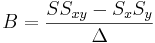
The correlation coefficient is used to determined whether or not there is a correlation within your data set. Once a correlation has been established, the actual relationship can be determined by carrying out a linear regression. The first step in performing a linear regression is calculating the slope and intercept:

\[\mathit{Slope} = \frac{n\sum_i X_iY_i -\sum_i X_i \sum_j Y_j }

ParseError: EOF expected (click for details)

Callstack:
    at (Bookshelves/Industrial_and_Systems_Engineering/Chemical_Process_Dynamics_and_Controls_(Woolf)/13:_Statistics_and_Probability_Background/13.01:_Basic_statistics-_mean_median_average_standard_deviation_z-scores_and_p-value), /content/body/div[2]/div[12]/p[2]/span, line 1, column 2

\nonumber \]

\[\mathrm{Intercept} = \frac{(\sum_i X_i^2)\sum_i(Y_i)-\sum_i X_i\sum_i X_iY_i }

ParseError: invalid ArgList (click for details)

Callstack:
    at (Bookshelves/Industrial_and_Systems_Engineering/Chemical_Process_Dynamics_and_Controls_(Woolf)/13:_Statistics_and_Probability_Background/13.01:_Basic_statistics-_mean_median_average_standard_deviation_z-scores_and_p-value), /content/body/div[2]/div[12]/p[3]/span, line 1, column 3

\nonumber \]

Once the slope and intercept are calculated, the uncertainty within the linear regression needs to be applied. To calculate the uncertainty, the standard error for the regression line needs to be calculated.

\[S=\sqrt{\frac{1}{n-2}\left(\left(\sum_{i} Y_{i}^{2}\right)-\text { intercept } \sum Y_{i}-\operatorname{slope}\left(\sum_{i} Y_{i} X_{i}\right)\right)}\nonumber \]

The standard error can then be used to find the specific error associated with the slope and intercept:

\[S_{\text {slope }}=S \sqrt{\frac{n}{n \sum_{i} X_{i}^{2}-\left(\sum_{i} X_{i}\right)^{2}}}\nonumber \]

\[S_{\text {intercept }}=S \sqrt{\frac{\sum\left(X_{i}^{2}\right)}{n\left(\sum X_{i}^{2}\right)-\left(\sum_{i} X_{i} Y_{i}\right)^{2}}}\nonumber \]

Once the error associated with the slope and intercept are determined a confidence interval needs to be applied to the error. A confidence interval indicates the likelihood of any given data point, in the set of data points, falling inside the boundaries of the uncertainty. 

\[\beta=slope\pm\Delta slope\simeq slope\pm t^*S_{slope} \nonumber \]

\[\alpha=intercept\pm\Delta intercept\simeq intercept\pm t^*S_{intercept} \nonumber \]

Now that the slope, intercept, and their respective uncertainties have been calculated, the equation for the linear regression can be determined.

\[Y = βX + α\nonumber \]

Z-Scores

A z-score (also known as z-value, standard score, or normal score) is a measure of the divergence of an individual experimental result from the most probable result, the mean. Z is expressed in terms of the number of standard deviations from the mean value.

\[z=\frac{X-\mu}{\sigma} \label{6} \]

• X = ExperimentalValue
• μ = Mean
• σ = StandardDeviation

Z-scores assuming the sampling distribution of the test statistic (mean in most cases) is normal and transform the sampling distribution into a standard normal distribution. As explained above in the section on sampling distributions, the standard deviation of a sampling distribution depends on the number of samples. Equation (6) is to be used to compare results to one another, whereas equation (7) is to be used when performing inference about the population.

Whenever using z-scores it is important to remember a few things:

• Z-scores normalize the sampling distribution for meaningful comparison.
• Z-scores require a large amount of data.
• Z-scores require independent, random data.

\[z_{o b s}=\frac{X-\mu}{\frac{\sigma}{\sqrt{n}}} \label{7} \]

• n = SampleNumber

P-Value

A p-value is a statistical value that details how much evidence there is to reject the most common explanation for the data set. It can be considered to be the probability of obtaining a result at least as extreme as the one observed, given that the null hypothesis is true. In chemical engineering, the p-value is often used to analyze marginal conditions of a system, in which case the p-value is the probability that the null hypothesis is true.

The null hypothesis is considered to be the most plausible scenario that can explain a set of data. The most common null hypothesis is that the data is completely random, that there is no relationship between two system results. The null hypothesis is always assumed to be true unless proven otherwise. An alternative hypothesis predicts the opposite of the null hypothesis and is said to be true if the null hypothesis is proven to be false.

The following is an example of these two hypotheses:

4 students who sat at the same table during in an exam all got perfect scores.

• Null Hypothesis: The lack of a score deviation happened by chance.
• Alternative Hypothesis: There is some other reason that they all received the same score.

If it is found that the null hypothesis is true then the Honor Council will not need to be involved. However, if the alternative hypothesis is found to be true then more studies will need to be done in order to prove this hypothesis and learn more about the situation.

As mentioned previously, the p-value can be used to analyze marginal conditions. In this case, the null hypothesis is that there is no relationship between the variables controlling the data set. For example:

• Runny feed has no impact on product quality
• Points on a control chart are all drawn from the same distribution
• Two shipments of feed are statistically the same

The p-value proves or disproves the null hypothesis based on its significance. A p-value is said to be significant if it is less than the level of significance, which is commonly 5%, 1% or .1%, depending on how accurate the data must be or stringent the standards are. For example, a health care company may have a lower level of significance because they have strict standards. If the p-value is considered significant (is less than the specified level of significance), the null hypothesis is false and more tests must be done to prove the alternative hypothesis.

Upon finding the p-value and subsequently coming to a conclusion to reject the Null Hypothesis or fail to reject the Null Hypothesis, there is also a possibility that the wrong decision can be made. If the decision is to reject the Null Hypothesis and in fact the Null Hypothesis is true, a type 1 error has occurred. The probability of a type one error is the same as the level of significance, so if the level of significance is 5%, "the probability of a type 1 error" is .05 or 5%. If the decision is to fail to reject the Null Hypothesis and in fact the Alternative Hypothesis is true, a type 2 error has just occurred. With respect to the type 2 error, if the Alternative Hypothesis is really true, another probability that is important to researchers is that of actually being able to detect this and reject the Null Hypothesis. This probability is known as the power (of the test) and it is defined as 1 - "probability of making a type 2 error."

If an error occurs in the previously mentioned example testing whether there is a relationship between the variables controlling the data set, either a type 1 or type 2 error could lead to a great deal of wasted product, or even a wildly out-of-control process. Therefore, when designing the parameters for hypothesis testing, researchers must heavily weigh their options for level of significance and power of the test. The sensitivity of the process, product, and standards for the product can all be sensitive to the smallest error.

Important Note About Significant P-values

If a P-value is greater than the applied level of significance, and the null hypothesis should not just be blindly accepted. Other tests should be performed in order to determine the true relationship between the variables which are being tested. More information on this and other misunderstandings related to P-values can be found at P-values: Frequent misunderstandings.

Calculation

There are two ways to calculate a p-value. The first method is used when the z-score has been calculated. The second method is used with the Fisher’s exact method and is used when analyzing marginal conditions.

First Method: Z-Score

The method for finding the P-Value is actually rather simple. First calculate the z-score and then look up its corresponding p-value using the standard normal table.

This table can be found here: Media:Group_G_Z-Table.xls

This value represents the likelihood that the results are not occurring because of random errors but rather an actual difference in data sets.

To read the standard normal table, first find the row corresponding to the leading significant digit of the z-value in the column on the lefthand side of the table. After locating the appropriate row move to the column which matches the next significant digit.

Example:
If your z-score = 1.13

Follow the rows down to 1.1 and then across the columns to 0.03. The P-value is the highlighted box with a value of 0.87076.

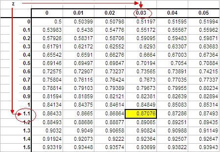
Values in the table represent area under the standard normal distribution curve to the left of the z-score.

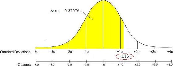
Using the previous example:

Z-score = 1.13, P-value = 0.87076 is graphically represented below.

Second Method: Fisher's Exact

In the case of analyzing marginal conditions, the P-value can be found by summing the Fisher's exact values for the current marginal configuration and each more extreme case using the same marginals. For information about how to calculate Fisher's exact click the following link:Discrete_Distributions:_hypergeometric,_binomial,_and_poisson#Fisher.27s_exact

Chi-Squared Test

A Chi-Squared test gives an estimate on the agreement between a set of observed data and a random set of data that you expected the measurements to fit. Since the observed values are continuous, the data must be broken down into bins that each contain some observed data. Bins can be chosen to have some sort of natural separation in the data. If none of these divisions exist, then the intervals can be chosen to be equally sized or some other criteria.

The calculated chi squared value can then be correlated to a probability using excel or published charts. Similar to the Fisher's exact, if this probability is greater than 0.05, the null hypothesis is true and the observed data is not significantly different than the random.

Calculating Chi Squared

The Chi squared calculation involves summing the distances between the observed and random data. Since this distance depends on the magnitude of the values, it is normalized by dividing by the random value

\[\chi^2 =\sum_{k=1}^N \frac{(observed-random)^2}{random}\nonumber \]

or if the error on the observed value (sigma) is known or can be calculated:

\[\chi^{2}=\sum_{k=1}^{N}\left(\frac{\text { observed }-\text { theoretical }}{\text { sigma }}\right)^{2}\nonumber \]

Detailed Steps to Calculate Chi Squared by Hand

Calculating Chi squared is very simple when defined in depth, and in step-by-step form can be readily utilized for the estimate on the agreement between a set of observed data and a random set of data that you expected the measurements to fit. Given the data:

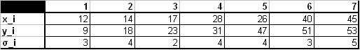
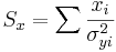
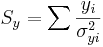
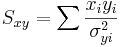
Step 1: Find

\[\chi_o^2 =\sum_{i} \frac{(y_i-A-Bx_i)^2}{\sigma_{yi}^2}\nonumber \]

When:

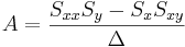
\[\Delta=SS_{xx}-(S_x)^2\,\!\nonumber \]

The Excel function CHITEST(actual_range, expected_range) also calculates the value. The two inputs represent the range of data the actual and expected data, respectively.

Step 2: Find the Degrees of Freedom

When: df = Degrees of Freedom

• n = number of observations
• k = the number of constraints

Step 3: Find

\[\tilde{\chi}_o^2\nonumber \]= the established value of obtained in an experiment with df degrees of freedom

Step 4: Find 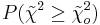using Excel or published charts.

The Excel function CHIDIST(x,df) provides the p-value, where x is the value of the chi-squared statistic and df is the degrees of freedom. Note: Excel gives only the p-value and not the value of the chi-square statistic.

= the probability of getting a value of that is as large as the established

Step 5: Compare the probability to the significance level (i.e. 5% or 0.05), if this probability is greater than 0.05, the null hypothesis is true and the observed data is not significantly different than the random. A probability smaller than 0.05 is an indicator of independence and a significant difference from the random.

Chi Squared Test versus Fisher's Exact

• For small sample sizes, the Chi Squared Test will not always produce an accurate probability. However, for a random null, the Fisher's exact, like its name, will always give an exact result.

• Chi Squared will not be correct when:

1. fewer than 20 samples are being used
2. if an expected number is 5 or below and there are between 20 and 40 samples

• For large contingency tables and expected distributions that are not random, the p-value from Fisher's Exact can be a difficult to compute, and Chi Squared Test will be easier to carry out.

Binning in Chi Squared and Fisher’s Exact Tests

When performing various statistical analyzes you will find that Chi-squared and Fisher’s exact tests may require binning, whereas ANOVA does not. Although there is no optimal choice for the number of bins (k), there are several formulas which can be used to calculate this number based on the sample size (N). One such example is listed below:

\[k = 1 + log_2N \nonumber \nonumber \]

Another method involves grouping the data into intervals of equal probability or equal width. The first approach in which the data is grouped into intervals of equal probability is generally more acceptable since it handles peaked data much better. As a stipulation, each bin should contain at least 5 or more data points, so certain adjacent bins sometimes need to be joined together for this condition to be satisfied. Identifying the number the bins to use is important, but it is even more important to be able to note which situations call for binning. Some Chi-squared and Fisher's exact situations are listed below:

• Analysis of a continuous variable:

This situation will require binning. The idea is to divide the range of values of the variable into smaller intervals called bins.

• Analysis of a discrete variable:

Binning is unnecessary in this situation. For instance, a coin toss will result in two possible outcomes: heads or tails. In tossing ten coins, you can simply count the number of times you received each possible outcome. This approach is similar to choosing two bins, each containing one possible result.

• Examples of when to bin, and when not to bin:

• You have twenty measurements of the temperature inside a reactor: as temperature is a continuous variable, you should bin in this case. One approach might be to determine the mean (X) and the standard deviation (σ) and group the temperature data into four bins: T < X – σ, X – σ < T < X, X < T < X + σ, T > X + σ
• You have twenty data points of the heater setting of the reactor (high, medium, low): since the heater setting is discrete, you should not bin in this case.

Example \(\PageIndex{1}\)

Say we have a reactor with a mean pressure reading of 100 and standard deviation of 7 psig. Calculate the probability of measuring a pressure between 90 and 105 psig.

Solution

To do this we will make use of the z-scores.

\[\operatorname{Pr}(a \leq z \leq b)=F(b)-F(a)=F\left(\frac{b-\mu}{\sigma}\right)-F\left(\frac{a-\mu}{\sigma}\right)\nonumber \]

where \(a\) is the lower bound and \(b\) is the upper bound

Substitution of z-transformation equation (3)

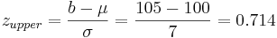
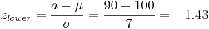
Look up z-score values in a standard normal table. Media:Group_G_Z-Table.xls

So:

= 0.76155 - 0.07636

= 0.68479.

The probability of measuring a pressure between 90 and 105 psig is 0.68479.

A graphical representation of this is shown below. The shaded area is the probability

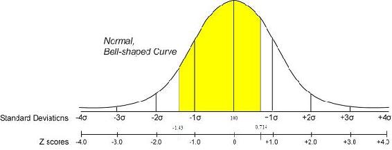
Alternate Solution

We can also solve this problem using the probability distribution function (PDF). This can be done easily in Mathematica as shown below. More information about the PDF is and how it is used can be found in the Continuous Distribution article

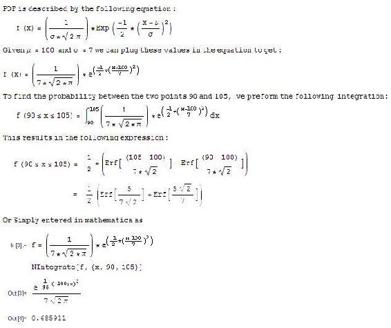
As you can see the the outcome is approximately the same value found using the z-scores.

Example \(\PageIndex{2}\)

You are a quality engineer for the pharmaceutical company “Headache-b-gone.” You are in charge of the mass production of their children’s headache medication. The average weight of acetaminophen in this medication is supposed to be 80 mg, however when you run the required tests you find that the average weight of 50 random samples is 79.95 mg with a standard deviation of .18.

1. Identify the null and alternative hypothesis.
2. Under what conditions is the null hypothesis accepted?
3. Determine if these differences in average weight are significant.

Solution

a)

• Null hypothesis: This is the claimed average weight where H_o=80 mg
• Alternative hypothesis: This is anything other than the claimed average weight (in this case H_a<80)

b) The null hypothesis is accepted when the p-value is greater than .05.

c) We first need to find Z_obs using the equation below:

\[z_{o b s}=\frac{X-\mu}{\frac{\sigma}{\sqrt{n}}}\nonumber \]

Where n is the number of samples taken.

\[z_{o b s}=\frac{79.95-80}{\frac{.18}{\sqrt{50}}}=-1.96\nonumber \]

Using the z-score table provided in earlier sections we get a p-value of .025. Since this value is less than the value of significance (.05) we reject the null hypothesis and determine that the product does not reach our standards.

Example \(\PageIndex{3}\)

15 students in a controls class are surveyed to see if homework impacts exam grades. The following distribution is observed.

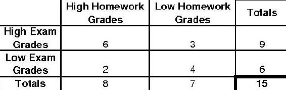
Determine the p-value and if the null hypothesis (Homework does not impact Exams) is significant by a 5% significance level using the P-fisher method.

Solution

To find the p-value using the p-fisher method, we must first find the p-fisher for the original distribution. Then, we must find the p-fisher for each more extreme case. The p-fisher for the original distribution is as follows.

\[p_{\text {fisher }}=\frac{9 ! 6 ! 8 ! 7 !}{15 ! 6 ! 3 ! 2 ! 4 !}=0.195804 \nonumber \]

To find the more extreme case, we will gradually decrease the smallest number to zero. Thus, our next distribution would look like the following.

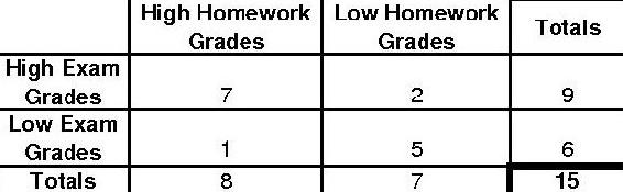
The p-fisher for this distribution will be as follows.

\[p_{\text {fisher }}=\frac{9 ! 6 ! 8 ! 7 !}{15 ! 7 ! 2 ! 1 ! 5 !}=0.0335664 \nonumber \]

The final extreme case will look like this.

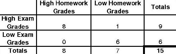
The p-fisher for this distribution will be as follows.

\[p_{\text {fisher }}=\frac{9 ! 6 ! 8 ! 7 !}{15 ! 8 ! 1 ! 0 ! 6 !}=0.0013986\nonumber \]

Since we have a 0 now in the distribution, there are no more extreme cases possible. To find the p-value we will sum the p-fisher values from the 3 different distributions.

\[p_{value} = 0.195804 + 0.0335664 + 0.0013986 = 0.230769\nonumber \]

Because p-value=0.230769 we cannot reject the null hypothesis on a 5% significance level.

Application: What do p-values tell us?

Population Example

Out of a random sample of 400 students living in the dormitory (group A), 134 students caught a cold during the academic school year. Out of a random sample of 1000 students living off campus (group B), 178 students caught a cold during this same time period.

Population table

\[\begin{array}{llll} 
& \text { Graup A } & \text { Group B } & \\
\text { Sick } & a=134 & b=178 & a+b=312 \\
\text { Not Sick } & c=266 & d=822 & c+d=1088 \\
& a+c=400 & b+d=1000 & a+b+c+d=1400
\end{array}\nonumber \]

Fisher's Exact:

\[p_{f}=\frac{(a+b) !(c+d) !(a+c) !(b+d) !}{(a+b+c+d) ! a ! b ! c ! d !}\nonumber \]

Solve:

\[p_{f}=\frac{(312) !(1088) !(400) !(1000) !}{(1400) ! 134 ! 178 ! 266 ! 822 !}\nonumber \]

p_f = 2.28292 * 10 ^{− 10}

Comparison and interpretation of p-value at the 95% confidence level

This value is very close to zero which is much less than 0.05. Therefore, the number of students getting sick in the dormitory is significantly higher than the number of students getting sick off campus. There is more than a 95% chance that this significant difference is not random. Statistically, it is shown that this dormitory is more condusive for the spreading of viruses. With the knowledge gained from this analysis, making changes to the dormitory may be justified. Perhaps installing sanitary dispensers at common locations throughout the dormitory would lower this higher prevalence of illness among dormitory students. Further research may determine more specific areas of viral spreading by marking off several smaller populations of students living in different areas of the dormitory. This model of significance testing is very useful and is often applied to a multitude of data to determine if discrepancies are due to chance or actual differences between compared samples of data. As you can see, purely mathematical analyses such as these often lead to physical action being taken, which is necessary in the field of Medicine, Engineering, and other scientific and non-scientific venues.

Exercise \(\PageIndex{1}\)

You are given the following set of data: {1,2,3,5,5,6,7,7,7,9,12} What is the mean, median and mode for this set of data? And then the z value of a data point of 7?

1. 5.82, 6, 7, 0.373
2. 6, 7, 5.82, 6.82
3. 7, 6, 5, 0.373
4. 7, 6, 5.82, 3.16

Answer

a

Exercise \(\PageIndex{2}\)

What is n and the standard deviation for the above set of data {1,2,3,5,5,6,7,7,7,9,12}? And then consulting the table from above, what is the p-value for the data "12"?

1. 12, 3.16, 5.82
2. 7, 3.16, 0.83
3. 11, 3.16, 0.97
4. 11, 5.82, 0

Answer

c

References

• Woolf P., Keating A., Burge C., and Michael Y.. "Statistics and Probability Primer for Computational Biologists". Massachusetts Institute of Technology, BE 490/ Bio7.91, Spring 2004
• Smith W. and Gonic L. "Cartoon Guide to Statistics". Harper Perennial, 1993.
• Taylor, J. "An Introduction to Error Analysis". Sausalito, CA: University Science Books, 1982.
• http://www.fourmilab.ch/rpkp/experiments/analysis/zCalc.html