13.5: Bayesian Network Theory

Introduction

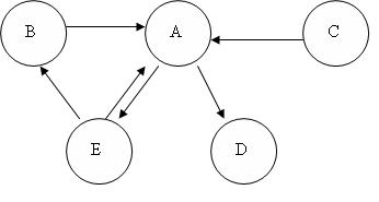
Bayesian network theory can be thought of as a fusion of incidence diagrams and Bayes’ theorem. A Bayesian network, or belief network, shows conditional probability and causality relationships between variables. The probability of an event occurring given that another event has already occurred is called a conditional probability. The probabilistic model is described qualitatively by a directed acyclic graph, or DAG. The vertices of the graph, which represent variables, are called nodes. The nodes are represented as circles containing the variable name. The connections between the nodes are called arcs, or edges. The edges are drawn as arrows between the nodes, and represent dependence between the variables. Therefore, for any pairs of nodes indicate that one node is the parent of the other so there are no independence assumptions. Independence assumptions are implied in Bayesian networks by the absence of a link. Here is a sample DAG:

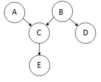
The node where the arc originates is called the parent, while the node where the arc ends is called the child. In this case, A is a parent of C, and C is a child of A. Nodes that can be reached from other nodes are called descendents. Nodes that lead a path to a specific node are called ancestors. For example, C and E are descendents of A, and A and C are ancestors of E. There are no loops in Bayesian networks, since no child can be its own ancestor or descendent. Bayesian networks will generally also include a set of probability tables, stating the probabilities for the true/false values of the variables. The main point of Bayesian Networks is to allow for probabilistic inference to be performed. This means that the probability of each value of a node in the Bayesian network can be computed when the values of the other variables are known. Also, because independence among the variables is easy to recognize since conditional relationships are clearly defined by a graph edge, not all joint probabilities in the Bayesian system need to be calculated in order to make a decision.

Joint Probability Distributions

Joint probability is defined as the probability that a series of events will happen concurrently. The joint probability of several variables can be calculated from the product of individual probabilities of the nodes:

\[\mathrm{P}\left(X_{1}, \ldots, X_{n}\right)=\prod_{i=1}^{n} \mathrm{P}\left(X_{i} \mid \text { parents }\left(X_{i}\right)\right) \nonumber \]

Using the sample graph from the introduction, the joint probability distribution is:

\[P(A, B, C, D, E)=P(A) P(B) P(C \mid A, B) P(D \mid B) P(E \mid C) \nonumber \]

If a node does not have a parent, like node A, its probability distribution is described as unconditional. Otherwise, the local probability distribution of the node is conditional on other nodes.

Equivalence Classes

Each Bayesian network belongs to a group of Bayesian networks known as an equivalence class. In a given equivalence class, all of the Bayesian networks can be described by the same joint probability statement. As an example, the following set of Bayesian networks comprises an equivalence class:

Network 1

Network 2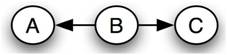

Network 3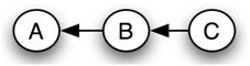

The causality implied by each of these networks is different, but the same joint probability statement describes them all. The following equations demonstrate how each network can be created from the same original joint probability statement:

Network 1

\[P(A, B, C)=P(A) P(B \mid A) P(C \mid B) \nonumber \]

Network 2

\[\begin{align*} P(A, B, C) &=P(A) P(B \mid A) P(C \mid B) \\[4pt] &=P(A) \frac{P(A \mid B) P(B)}{P(A)} P(C \mid B) \\[4pt] &=P(A \mid B) P(B) P(C \mid B) \end{align*} \nonumber \]

Network 3

Starting now from the statement for Network 2

\[\begin{align*} P(A, B, C) &=P(A \mid B) P(B) P(C \mid B) \\[4pt] &=P(A \mid B) P(B) \frac{P(B \mid C) P(C)}{P(B)} \\[4pt] &=P(A \mid B) P(B \mid C) P(C)\end{align*} \nonumber \]

All substitutions are based on Bayes rule.

The existence of equivalence classes demonstrates that causality cannot be determined from random observations. A controlled study – which holds some variables constant while varying others to determine each one’s effect – is necessary to determine the exact causal relationship, or Bayesian network, of a set of variables.

Bayes' Theorem

Bayes' Theorem, developed by the Rev. Thomas Bayes, an 18th century mathematician and theologian, it is expressed as:

\[P(H \mid E, c)=\frac{P(H \mid c) \cdot P(E \mid H, c)}{P(E \mid c)} \nonumber \]

where we can update our belief in hypothesis \(H\) given the additional evidence \(E\) and the background information \(c\). The left-hand term, \(P(H|E,c)\) is known as the "posterior probability," or the probability of H after considering the effect of E given c. The term \(P(H|c)\) is called the "prior probability" of \(H\) given c alone. The term \(P(E|H,c)\) is called the "likelihood" and gives the probability of the evidence assuming the hypothesis \(H\) and the background information \(c\) is true. Finally, the last term \(P(E|c)\) is called the "expectedness", or how expected the evidence is given only \(c\). It is independent of \(H\) and can be regarded as a marginalizing or scaling factor.

It can be rewritten as

\[P(E \mid c)=\sum_{i} P\left(E \mid H_{i}, c\right) \cdot P\left(H_{i} \mid c\right) \nonumber \]

where i denotes a specific hypothesis H_i, and the summation is taken over a set of hypotheses which are mutually exclusive and exhaustive (their prior probabilities sum to 1).

It is important to note that all of these probabilities are conditional. They specify the degree of belief in some proposition or propositions based on the assumption that some other propositions are true. As such, the theory has no meaning without prior determination of the probability of these previous propositions.

Bayes' Factor

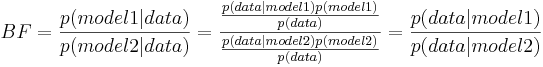
In cases when you are unsure about the causal relationships between the variables and the outcome when building a model, you can use Bayes Factor to verify which model describes your data better and hence determine the extent to which a parameter affects the outcome of the probability. After using Bayes' Theorem to build two models with different variable dependence relationships and evaluating the probability of the models based on the data, one can calculate Bayes' Factor using the general equation below:

\[B F=\frac{p(\text {model} 1 \mid \text {data})}{p(\text {model} 2 \mid \text {data})}=\frac{\frac{p(\text {data} \mid \text {model} 1) p(\text {model} 1)}{p(\text {data})}}{\frac{p(\text {data} \mid \operatorname{model} 2) p(\operatorname{model} 2)}{p(\text {data})}}=\frac{p(\text {data} \mid \text {model} 1)}{p(\text {data} \mid \operatorname{model} 2)} \nonumber \]

The basic intuition is that prior and posterior information are combined in a ratio that provides evidence in favor of one model verses the other. The two models in the Bayes' Factor equation represent two different states of the variables which influence the data. For example, if the data being studied are temperature measurements taken from multiple sensors, Model 1 could be the probability that all sensors are functioning normally, and Model 2 the probability that all sensors have failed. Bayes' Factors are very flexible, allowing multiple hypotheses to be compared simultaneously.

BF values near 1, indicate that the two models are nearly identical and BF values far from 1 indicate that the probability of one model occurring is greater than the other. Specifically, if BF is > 1, model 1 describes your data better than model 2. IF BF is < 1, model 2 describes the data better than model 1. In our example, if a Bayes' factor of 5 would indicate that given the temperature data, the probability of the sensors functioning normally is five times greater than the probability that the senors failed. A table showing the scale of evidence using Bayes Factor can be found below:

scale of Evidence for Bayes factors

\[\begin{array}{|c|c|}
\hline \text { Bayes factor } & \text { Interpretat on } \\
\hline \text { B.F. }<1 / 10 & \text { Strong evidence for Model } 2 \\
1 / 10<\text { B.F. }<1 / 3 & \text { Moderate evidence for Model } 2 \\
\hline 1 / 3<\text { B.F. }<1 & \text { Weak evidence for Mocel } 2 \\
\hline 1<\text { B.F. }<3 & \text { Weak evidence for Model } 1 \\
\hline 3<\text { B.F F } 10 & \text { Moderate evidence for Model } 1 \\
\hline \text { B.F. }>10 & \text { Strong evidence for Model } 1 \\
\hline
\end{array}\]

Although Bayes' Factors are rather intuitive and easy to understand, as a practical matter they are often quite difficult to calculate. There are alternatives to Bayes Factor for model assessment such as the Bayesian Information Criterion (BIC).

The formula for the BIC is:

\[-2 \cdot \ln p(x \mid k) \approx \mathrm{BIC}=-2 \cdot \ln L+k \ln (n). \nonumber \]

• x = the observed data; n = the number of data points in x, the number of observations, or equivalently, the sample size;
• k = the number of free parameters to be estimated. If the estimated model is a linear regression, k is the number of regressors, including the constant; p(x|k) = the likelihood of the observed data given the number of parameters;
• L = the maximized value of the likelihood function for the estimated model.

This statistic can also be used for non-nested models. For further information on Bayesian Information Criterion, please refer to:

Advantages and Limitations of Bayesian Networks

The advantages of Bayesian Networks are as follows:

• Bayesian Networks visually represent all the relationships between the variables in the system with connecting arcs.
• It is easy to recognize the dependence and independence between various nodes.
• Bayesian networks can handle situations where the data set is incomplete since the model accounts for dependencies between all variables.
• Bayesian networks can maps scenarios where it is not feasible/practical to measure all variables due to system constraints (costs, not enough sensors, etc.)
• Help to model noisy systems.
• Can be used for any system model - from all known parameters to no known parameters.

The limitations of Bayesian Networks are as follows:

• All branches must be calculated in order to calculate the probability of any one branch.
• The quality of the results of the network depends on the quality of the prior beliefs or model. A variable is only a part of a Bayesian network if you believe that the system depends on it.
• Calculation of the network is NP-hard (nondeterministic polynomial-time hard), so it is very difficult and possibly costly.
• Calculations and probabilities using Baye's rule and marginalization can become complex and are often characterized by subtle wording, and care must be taken to calculate them properly.

Inference

Inference is defined as the process of deriving logical conclusions based on premises known or assumed to be true. One strength of Bayesian networks is the ability for inference, which in this case involves the probabilities of unobserved variables in the system. When observed variables are known to be in one state, probabilities of other variables will have different values than the generic case. Let us take a simple example system, a television. The probability of a television being on while people are home is much higher than the probability of that television being on when no one is home. If the current state of the television is known, the probability of people being home can be calculated based on this information. This is difficult to do by hand, but software programs that use Bayesian networks incorporate inference. One such software program, Genie, is introduced in Learning and analyzing Bayesian networks with Genie.

Marginalization

Marginalization of a parameter in a system may be necessary in a few instances:

• If the data for one parameter (P1) depends on another, and data for the independent parameter is not provided.
• If a probability table is given in which P1 is dependent upon two other system parameters, but you are only interested in the effect of one of the parameters on P1.

Imagine a system in which a certain reactant (R) is mixed in a CSTR with a catalyst (C) and results in a certain product yield (Y). Three reactant concentrations are being tested (A, B, and C) with two different catalysts (1 and 2) to determine which combination will give the best product yield. The conditional probability statement looks as such:

\[P(R, C, Y)=P(R) P(C) P(Y \mid R, C) \nonumber \]

The probability table is set up such that the probability of certain product yield is dependent upon the reactant concentration and the catalyst type. You want to predict the probability of a certain product yield given only data you have for catalyst type. The concentration of reactant must be marginalized out of P(Y|R,C) to determine the probability of the product yield without knowing the reactant concentration. Thus, you need to determine P(Y|C). The marginalization equation is shown below:

\[P(Y \mid C)=\sum_{i} P\left(Y \mid R_{i}, C\right) P\left(R_{i}\right) \nonumber \]

where the summation is taken over reactant concentrations A, B, and C.

The following table describes the probability that a sample is tested with reactant concentration A, B, or C:

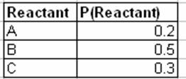
This next table describes the probability of observing a yield - High (H), Medium (M), or Low (L) - given the reactant concentration and catalyst type:

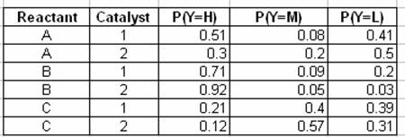
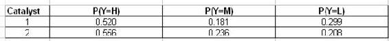
The final two tables show the calculation for the marginalized probabilities of yield given a catalyst type using the marginalization equation:

Dynamic Bayesian Networks

The static Bayesian network only works with variable results from a single slice of time. As a result, a static Bayesian network does not work for analyzing an evolving system that changes over time. Below is an example of a static Bayesian network for an oil wildcatter:

www.norsys.com/netlibrary/index.htm

An oil wildcatter must decide either to drill or not. However, he needs to determine if the hole is dry, wet or soaking. The wildcatter could take seismic soundings, which help determine the geological structure at the site. The soundings will disclose whether the terrain below has no structure, which is bad, or open structure that's okay, or closed structure, which is really good. As you can see this example does not depend on time.

Dynamic Bayesian Network (DBN) is an extension of Bayesian Network. It is used to describe how variables influence each other over time based on the model derived from past data. A DBN can be thought as a Markov chain model with many states or a discrete time approximation of a differential equation with time steps.

An example of a DBN, which is shown below, is a frictionless ball bouncing between two barriers. At each time step the position and velocity changes.

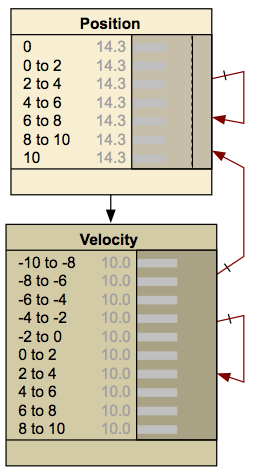
www.norsys.com/netlibrary/index.htm

An important distinction must be made between DBNs and Markov chains. A DBN shows how variables affect each other over time, whereas a Markov chain shows how the state of the entire system evolves over time. Thus, a DBN will illustrate the probabilities of one variable changing another, and how each of the individual variables will change over time. A Markov chain looks at the state of a system, which incorporates the state of each individual variable making up the system, and shows the probabilities of the system changing states over time. A Markov chain therefore incorporates all of the variables present in the system when looking at how said system evolves over time. Markov chains can be derived from DBNs, but each network represents different values and probabilities.

There are several advantages to creating a DBN. Once the network has been established between the time steps, a model can be developed based on this data. This model can then be used to predict future responses by the system. The ability to predict future responses can also be used to explore different alternatives for the system and determine which alternative gives the desired results. DBN's also provide a suitable environment for model predictive controllers and can be useful in creating the controller. Another advantage of DBN's is that they can be used to create a general network that does not depend on time. Once the DBN has been established for the different time steps, the network can be collapsed to remove the time component and show the general relationships between the variables.

A DBN is made up with interconnected time slices of static Bayesian networks. The nodes at certain time can affect the nodes at a future time slice, but the nodes in the future can not affect the nodes in the previous time slice. The causal links across the time slices are referred to as temporal links, the benefit of this is that it gives DBN an unambiguous direction of causality.

For the convenience of computation, the variables in DBN are assumed to have a finite number of states that the variable can have. Based on this, conditional probability tables can be constructed to express the probabilities of each child node derived from conditions of its parent nodes.

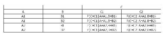
Node C from the sample DAG above would have a conditional probability table specifying the conditional distribution P(C|A,B). Since A and B have no parents, so it only require probability distributions P(A) and P(B). Assuming all the variables are binary, means variable A can only take on A1 and A2, variable B can only take on B1 and B2, and variable C can only take on C1 and C2. Below is an example of a conditional probability table of node C.

The conditional probabilities between observation nodes are defined using a sensor node. This sensor node gives conditional probability distribution of the sensor reading given the actual state of system. It embodies the accuracy of the system.

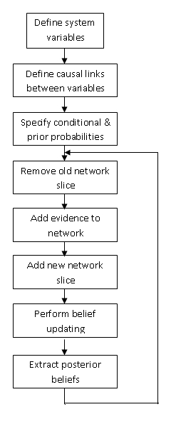
The nature of DBN usually results in a large and complex network. Thus to calculate a DBN, the outcome old time slice is summarized into probabilities that is used for the later slice. This provides a moving time frame and forms a DBN. When creating a DBN, temporal relationships between slices must be taken into account. Below is an implementation chart for DBN.

The graph below is a representation of a DBN. It represents the variables at two different time steps, t-1 and t. t-1, shown on the left, is the initial distribution of the variables. The next time step, t, is dependent on time step t-1. It is important to note that some of these variables could be hidden.

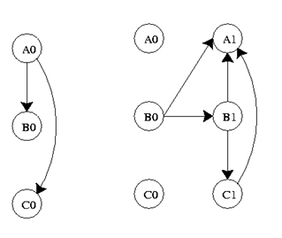
Where Ao, Bo, Co are initial states and Ai, Bi, Ci are future states where i=1,2,3,…,n.

The probability distribution for this DBN at time t is…

\[P\left(Z_{t} \mid Z_{t-1}\right)=\prod_{i=1}^{N} P\left(Z_{t}^{i} \mid \pi\left(Z_{t}^{i}\right)\right) \nonumber \]

If the process continues for a larger number of time steps, the graph will take the shape below.

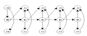
Its joint probability distribution will be...

\[P\left(Z_{1: T}\right)=\prod_{t=1}^{T} \prod_{i=1}^{N} P\left(Z_{t}^{i} \mid \pi\left(Z_{t}^{i}\right)\right) \nonumber \]

DBN’s are useful in industry because they can model processes where information is incomplete, or there is uncertainty. Limitations of DBN’s are that they do not always accurately predict outcomes and they can have long computational times.

The above illustrations are all examples of "unrolled" networks. An unrolled dynamic Bayesian network shows how each variable at one time step affects the variables at the next time step. A helpful way to think of unrolled networks is as visual representations of numerical solutions to differential equations. If you know the states of the variables at one point in time, and you know how the variables change with time, then you can predict what the state of the variables will be at any point in time, similar to using Euler's method to solve a differential equation. A dynamic Bayesian network can also be represented as a "rolled" network. A rolled network, unlike an unrolled network, shows each variables' effect on each other variable in one chart. For example, if you had an unrolled network of the form:

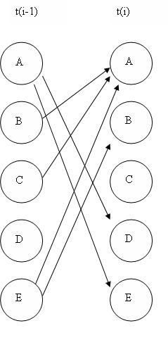
then you could represent that same network in a rolled form as:

If you examine each network, you will see that each one provides the exact same information as to how the variables all affect each other.

Applications

Bayesian networks are used when the probability that one event will occur depends on the probability that a previous event occurred. This is very important in industry because in many processes, variables have conditional relationships, meaning they are not independent of each other. Bayesian networks are used to model processes in a wide variety of applications. Some of these include…

1. Gene regulatory networks
2. Protein structure
3. Diagnosis of illness
4. Document classification
5. Image processing
6. Data fusion
7. Decision support systems
8. Gathering data for deep space exploration
9. Artificial Intelligence
10. Prediction of weather
11. On a more familiar basis, Bayesian networks are used by the friendly Microsoft office assistant to elicit better search results.\
12. Another use of Bayesian networks arises in the credit industry where an individual may be assigned a credit score based on age, salary, credit history, etc. This is fed to a Bayesian network which allows credit card companies to decide whether the person's credit score merits a favorable application.

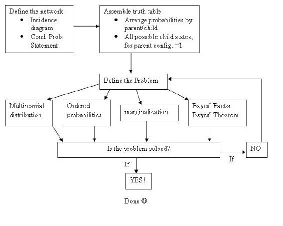
Summary: A General Solution Algorithm for the Perplexed

Given a Bayesian network problem and no idea where to start, just relax and try following the steps outlined below.

Step 1: What does my network look like? Which nodes are parents (and are they conditional or unconditional) and which are children? How would I model this as an incidence diagram and what conditional probability statement defines it?

Step 2: Given my network connectivity, how do I tabulate the probabilities for each state of my node(s) of interest? For a single column of probabilities (parent node), does the column sum to 1? For an array of probabilities (child node) with multiple possible states defined by the given combination of parent node states, do the rows sum to 1?

Step 3: Given a set of observed data (usually states of a child node of interest), and probability tables (aka truth tables), what problem am I solving?

• Probability of observing the particular configuration of data, order unimportant

Solution: Apply multinomial distribution

• Probability of observing the particular configuration of data in that particular order

Solution: Compute the probability of each individual observation, then take the product of these

• Probability of observing the data in a child node defined by 2 (or n) parents given only 1 (or n-1) of the parent nodes

Solution: Apply marginalization to eliminate other parent node

• Probability of a parent node being a particular state given data in the form of observed states of the child node

Solution: Apply Bayes' Theorem
Solve for Bayes' Factor to remove incalculable denominator terms generated by applying Bayes’ Theorem, and to compare the parent node state of interest to a base case, yielding a more meaningful data point

Step 4: Have I solved the problem? Or is there another level of complexity? Is the problem a combination of the problem variations listed in step 3?

• If problem is solved, call it a day and go take a baklava break
• If problem is not solved, return to step 3

Graphically:

Example \(\PageIndex{1}\)

A multipurpose alarm in a plant can be tripped in 2 ways. The alarm goes off if the reactor temperature is too high or the pressure in a storage tank is too high. The reactor temperature may be too high because of a low cooling water flow (1% probability), or because of an unknown side reaction (5% probability). The storage tank pressure might be too high because of a blockage in the outlet piping (2% probability). If the cooling water flow is low and there is a side reaction, then there is a 99% probability that a high temperature will occur. If the cooling water flow is normal and there is no side reaction, there is only a 3% probability a high temperature will occur. If there is a pipe blockage, a high pressure will always occur. If there is no pipe blockage, a high pressure will occur only 2% of the time.

Create a DAG for the situation above, and set up the probability tables needed to model this system. All the values required to fill in these tables are not given, so fill in what is possible and then indicate what further values need to be found.

Solution

The following probability tables describe the system, where CFL = Cold water flow is low, SR = Side reaction present, PB = Pipe is blocked, HT = High temperature, HP = High pressure, A = Alarm. T stands for true, or the event did occur. F stands for false, or the event did not occur. A blank space in a table indicates an area where further information is needed.

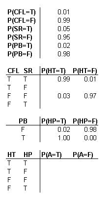
An advantage of using DAGs becomes apparent. For example, you can see that there is only a 3% chance that there is a high temperature situation given that both cold water flow is not low and that there is no side reaction.However, as soon as the cold water becomes low, you have at least a 94% chance of a high temperature alarm, regardless of whether or not a side reaction occurs. Conversely, the presence of a side reaction here only creates a 90% chance of alarm trigger. From the above probability calculations, one can estimate relative dominance of cause-and-effect triggers. For example you could now reasonably conjecture that the cold water being low is a more serious event than a side reaction.

Example \(\PageIndex{2}\)

The DAG given below depicts a different model in which the alarm will ring when activated by high temperature and/or coolant water pipe leakage in the reactor.

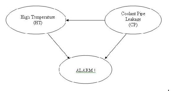
The table below shows the truth table and probabilities with regards to the different situations that might occur in this model.

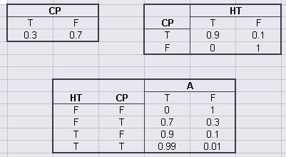
The joint probability function is:

\[P(A,HT,CP) = P(A | HT,CP)P(HT | CP)P(CP) \nonumber \]

A great feature of using the Bayesian network is that the probability of any situation can be calculated. In this example, write the statement that will describe the probability that the temperature is high in the reactor given that the alarm sounded.

Solution

\[\mathrm{P}(C P=T \mid \Delta=T)=\frac{\mathrm{P}(A=T, C P=T)}{\mathrm{P}(A=1)} [= \dfrac{\sum_{HTC[T,P]}P(A-T, HT, CP-T)}{\sum_{HT, CPC[T,P]}P(A=T, HT, CP)} \nonumber \]

Example \(\PageIndex{3}\)

Certain medications and traumas can both cause blood clots. A blood clot can lead to a stroke, heart attack, or it could simply dissolve on its own and have no health implications. Create a DAG that represents this situation.

Solution

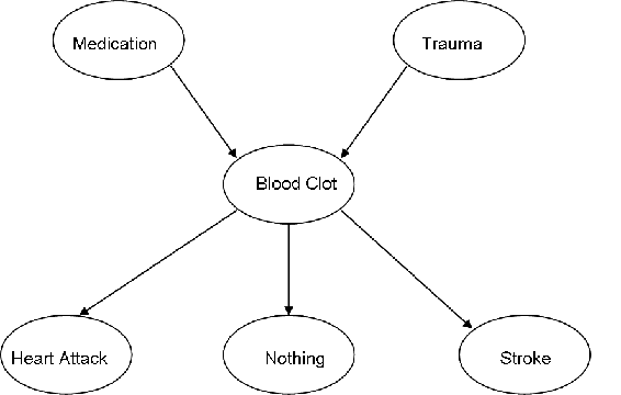
b. The following probability information is given where M = medication, T = trauma, BC = blood clot, HA = heart attack, N = nothing, and S = stroke. T stands for true, or this event did occur. F stands for false, or this event did not occur.

What is the probability that a person will develop a blood clot as a result of both medication and trauma, and then have no medical implications?

Answer

\[\mathrm{P}(\mathrm{N}, \mathrm{BC}, \mathrm{M}, \mathrm{T})=\mathrm{P}(\mathrm{N} \mid \mathrm{BC}) \mathrm{P}(\mathrm{BC} \mid \mathrm{M}, \mathrm{T}) \mathrm{P}(\mathrm{M}) \mathrm{P}(\mathrm{T})=(0.25)(0.95)(0.2)(0.05)=0.2375 \% \nonumber \]

Example \(\PageIndex{4}\)

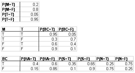
Suppose you were given the following data.

Catalyst	p(Catalyst)
A	0.40
B	0.60

Temperature	Catalyst	P(Yield = H)	P(Yield = M)	P(Yield = L)
H	A	0.51	0.08	0.41
H	B	0.30	0.20	0.50
M	A	0.71	0.09	0.20
M	B	0.92	0.05	0.03
L	A	0.21	0.40	0.39
L	B	0.12	0.57	0.31

How would you use this data to find p(yield|temp) for 9 observations with the following descriptions?

# Times Observed	Temperature	Yield
4x	H	H
2x	M	L
3x	L	H

An DAG of this system is below:

Solution

Marginalization! The state of the catalyst can be marginalized out using the following equation:

p(yield | temp) =	∑	p(yield | temp,cati)p(cati)
	i = A,B

The two tables above can be merged to form a new table with marginalization:

Temperature	P(Yield = H)	P(Yield = M)	P(Yield = L)
H	0.51*0.4 + 0.3*0.6 = 0.384	0.08*0.4 + 0.2*0.6 = 0.152	0.41*0.4 + 0.5*0.6 = 0.464
M	0.71*0.4 + 0.92*0.6 = 0.836	0.09*0.4 + 0.05*0.6 = 0.066	0.20*0.4 + 0.03*0.6 = 0.098
L	0.21*0.4 + 0.12*0.6 = 0.156	0.40*0.4 + 0.57*0.6 = 0.502	0.39*0.4 + 0.31*0.6 = 0.342

\[p(\text {yield} \mid \text {temp})=\frac{9 !}{4 ! 2 ! 3 !} *\left(0.384^{4} * 0.098^{2} * 0.156^{3}\right)=0.0009989 \nonumber \]

Example \(\PageIndex{5}\)

A very useful use of Bayesian networks is determining if a sensor is more likely to be working or broken based on current readings using the Bayesian Factor discussed earlier. Suppose there is a large vat in your process with large turbulent flow that makes it difficult to accurately measure the level within the vat. To help you use two different level sensors positioned around the tank that read whether the level is high, normal, or low. When you first set up the sensor system you obtained the following probabilities describing the noise of a sensor operating normally.

Tank Level (L)	p(S=High)	p(S=Normal)	p(S=Low)
Above Operating Level Range	0.80	0.15	0.05
Within Operating Level Range	0.15	0.75	0.10
Below Operating Level Range	0.10	0.20	0.70

When the sensor fails there is an equal chance of the sensor reporting high, normal, or low regardless of the actual state of the tank. The conditional probability table for a fail sensor then looks like:

Tank Level (L)	p(S=High)	p(S=Normal)	p(S=Low)
Above Operating Level Range	0.33	0.33	0.33
Within Operating Level Range	0.33	0.33	0.33
Below Operating Level Range	0.33	0.33	0.33

From previous data you have determined that when the process is acting normally, as you believe it is now, the tank will be operating above the level range 10% of the time, within the level range 85% of the time, and below the level range 5% of the time. Looking at the last 10 observations (shown below) you suspect that sensor 1 may be broken. Use Bayesian factors to determine the probability of sensor 1 being broken compared to both sensors working.

Sensor 1	Sensor 2
High	Normal
Normal	Normal
Normal	Normal
High	High
Low	Normal
Low	Normal
Low	Low
High	Normal
High	High
Normal	Normal

From the definition of the Bayesian Factor we get.

For this set we will use the probability that we get the data given based on the model.

If we consider model 1 both sensors working and model 2 sensor 2 being broken we can find the BF for this rather easily.

p(data | model 1) = p(s1 data | model 1)*p(s2 data | model 1)

For both sensors working properly:

The probability of the sensor giving each reading has to be calculated first, which can be found by summing the probability the tank will be at each level and multiplying by probability of getting a specific reading at that level for each level.

p(s1 = high | model 1) = [(.10)*(.80) + (.85)*(.15) + (.05)*(.10) = 0.2125

p(s1 = normal | model 1) = [(.10)*(.15) + (.85)*(.75) + (.05)*(.20) = 0.6625

p(s1 = low | model 1) = [(.10)*(.05) + (.85)*(.10) + (.05)*(.70) = 0.125

Probability of getting sensor 1's readings (assuming working normally)

p(s1data | model1) = (.2125)⁴ * (.6625)³ * (.125)³ = 5.450 * 10 ^{− 6}

The probability of getting each reading for sensor 2 will be the same since it is also working normally

p(s2data | model1) = (.2125)² * (.6625)⁷ * (.125)¹ = 3.162 * 10 ^{− 4}

p(data | model1) = (5.450 * 10 ^{− 6}) * (3.162 * 10 ^{− 4}) = 1.723 * 10 ^{− 9}

For sensor 1 being broken:

The probability of getting each reading now for sensor one will be 0.33.

p(s1data | model2) = (0.33)⁴ * (0.33)³ * (0.33)³ = 1.532 * 10 ^{− 5}

The probability of getting the readings for sensor 2 will be the same as model 1, since both models assume sensor 2 is acing normally.

p(data | model2) = (1.532 * 10 ^{− 5}) * (3.162 * 10 ^{− 4}) = 4.844 * 10 ^{− 9}

A BF factor between 1/3 and 1 means there is weak evidence that model 2 is correct.

True or False?

1. Is the other name for Bayesian Network the "Believer" Network?

2. The nodes in a Bayesian network can represent any kind of variable (latent variable, measured parameter, hypothesis..) and are not restricted to random variables.

3. Bayesian network theory is used in part of the modeling process for artificial intelligence.

Answers:

1. F

2. T

3. T

References

1. Aksoy, Selim. "Parametric Models Part IV: Bayesian Belief Networks." Spring 2007. <www.cs.bilkent.edu.tr/~saksoy/courses/cs551/slides/cs551_parametric4.pdf>
2. Ben-Gal, Irad. “BAYESIAN NETWORKS.” Department of Industrial Engineering. Tel-Aviv University. <http://www.eng.tau.ac.il/~bengal/BN.pdf>http://www.dcs.qmw.ac.uk/~norman/BBNs/BBNs.htm
3. Charniak, Eugene (1991). "Bayesian Networks without Tears", AI Magazine, p. 8.
4. Friedman, Nir, Linial, Michal, Nachman, Iftach, and Pe’er, Dana. “Using Bayesian Networks to Analyze Expression Data.” JOURNAL OF COMPUTATIONAL BIOLOGY, Vol. 7, # 3/4, 2000, Mary Ann Liebert, Inc. pp. 601–620 <www.sysbio.harvard.edu/csb/ramanathan_lab/iftach/papers/FLNP1Full.pdf>
5. Guo, Haipeng. "Dynamic Bayesian Networks." August 2002.<www.kddresearch.org/Groups/Probabilistic-Reasoning/258,1,Slide 1>
6. Neil, Martin, Fenton, Norman, and Tailor, Manesh. “Using Bayesian Networks to Model Expected and Unexpected Operational Losses.” Risk Analysis, Vol. 25, No. 4, 2005 <http://www.dcs.qmul.ac.uk/~norman/papers/oprisk.pdf>
7. Niedermayer, Daryle. “An Introduction to Bayesian Networks and their Contemporary Applications.” December 1, 1998. < www.niedermayer.ca/papers/bayesian/bayes.html>
8. Seeley, Rich. "Bayesian networks made easy". Application Development Trends. December 4, 2007 <www.adtmag.com/article.aspx?id=10271&page=>.
9. http://en.Wikipedia.org/wiki/Bayesian_network