4.4: Relationship to Matrix Norms

The singular value decomposition can be used to compute the induced 2-norm of a matrix A.

Theorem 4.2

\[\begin{aligned}
\|A\|_{2} & \triangleq \sup _{x \neq 0} \frac{\|A x\|_{2}}{\|x\|_{2}} \\
&=\sigma_{1} \\
&=\sigma_{\max }(A)
\end{aligned}\ \tag{4.21}\]

which tells us that the maximum amplification is given by the maximum singular value.

Proof

\[\begin{aligned}
\sup _{x \neq 0} \frac{\|A x\|_{2}}{\|x\|_{2}} &=\sup _{x \neq 0} \frac{\left\|U \Sigma V^{\prime} x\right\|_{2}}{\|x\|_{2}} \\
&=\sup _{x \neq 0} \frac{\left\|\Sigma V^{\prime} x\right\|_{2}}{\|x\|_{2}} \\
&=\sup _{y \neq 0} \frac{\|\Sigma y\|_{2}}{\|V y\|_{2}} \\
&=\sup _{y \neq 0} \frac{\left(\sum_{i=1}^{r} \sigma_{i}^{2}\left|y_{i}\right|^{2}\right)^{\frac{1}{2}}}{\left(\sum_{i=1}^{r}\left|y_{i}\right|^{2}\right)^{\frac{1}{2}}} \\
& \leq \sigma_{1}
\end{aligned}\nonumber\]

For \(y=\left[\begin{array}{lll}
1 & 0 & \cdots & 0
\end{array}\right]^{T},\|\Sigma y\|_{2}=\sigma_{1}\), and the supremum is attained. (Notice that this correponds to \(x = v_{1}\). Hence, \(Av_{1}=\sigma_{1}u_{1}.\)

Another application of the singular value decomposition is in computing the minimal amplification a full rank matrix exerts on elements with 2-norm equal to 1.

Theorem 4.3

Given \(A \in C^{m \times n}\), suppose \(rank(A) = n\). Then

\[\min _{\|x\|_{2}=1}\|A x\|_{2}=\sigma_{n}(A)\ \tag{4.22}\]

Note that if \(rank(A) < n\), then there is an \(x\) such that the minimum is zero (rewrite \(A\) in terms of its SVD to see this).

Proof

For any \(\|x\|_{2}=1\),

\[\begin{aligned}
\|A x\|_{2} &=\left\|U \Sigma V^{\prime} x\right\|_{2} \\
&=\left\|\Sigma V^{\prime} x\right\|_{2} \quad \text { (invariant under multiplication by unitary matrices) } \\
&=\|\Sigma y\|_{2}
\end{aligned}\nonumber\]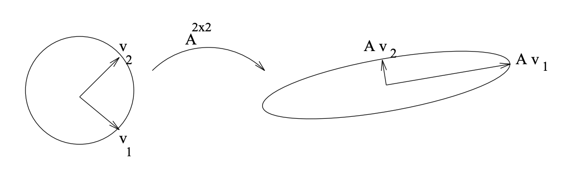

Figure \(\PageIndex{1}\): Graphical depiction of the mapping involving A^{2 \times 2}\). Note that \(Av_{1} = \sigma_{1} u_{1}\) and that \(Av_{2} = \sigma_{2} u_{2}\).

for \(y = V^{\prime}x\). Now

\[\begin{aligned}
\|\Sigma y\|_{2} &=\left(\sum_{i=1}^{n}\left|\sigma_{i} y_{i}\right|^{2}\right)^{\frac{1}{2}} \\
& \geq \sigma_{n}
\end{aligned}\nonumber\]

Note that the minimum is achieved for \(y=\left[\begin{array}{llll}
0 & 0 & \cdots & 0 &1
\end{array}\right]^{T}\); thus the proof is complete.

The Frobenius norm can also be expressed quite simply in terms of the singular values. We leave you to verify that

\[\begin{aligned}
\|A\|_{F} & \triangleq\left(\sum_{j=1}^{n} \sum_{i=1}^{m}\left|a_{i j}\right|^{2}\right)^{\frac{1}{2}} \\
&=\left(\operatorname{trace}\left(A^{\prime} A\right)\right)^{\frac{1}{2}} \\
&=\left(\sum_{i=1}^{r} \sigma_{i}^{2}\right)^{\frac{1}{2}}
\end{aligned}\ \tag{4.23}\]

Example 4.4 Matrix Inequality

We say \(A \leq B\), two square matrices, if

\[x^{\prime} A x \leq x^{\prime} B x \quad \text { for all } x \neq 0\nonumber\]

It follows that for any matrix A, not necessarily square,

\[\|A\|_{2} \leq \gamma \leftrightarrow A^{\prime} A \leq \gamma^{2} I.\nonumber\]