6.1: Introduction - Signals, Systems and Models

A system may be thought of as something that imposes constraints on - or enforces relationships among - a set of variables. This "system as constraints" point of view is very general and powerful. Rather more restricted, but still very useful and common, is the view of a system as a mapping from a set of input variables to a set of output variables; a mapping is evidently a very particular form of constraint.

A (behavioral) model lists the variables of interest (the "manifest" variables) and the constraints that they must satisfy. Any combination of variables that satisfies the constraints is possible or allowed, and is termed a behavior of the model.

To facilitate the specification of the constraints, one may introduce auxiliary ("latent") variables. One might then distinguish among the manifest behavior, latent behavior, and full behavior (manifest as well as latent).

For a dynamic model, the "variables" referred to above are actually signals that evolve as a function of time (and/or a function of other independent variables, e.g. space). We first need to specify a time axis \(\mathbb{T}\) (discrete, continuous, infinite, semi-infinite . . . ) and a signal space \(\mathbb{W}\), i.e. the space of values the signals live in at each time instant. A dynamic model for a set of signals \(\left\{w_{i}(t)\right\}\) is then completed by listing the constraints that the \(w_{i}(t)\) must satisfy. Any combination \(w(t)=\left[\begin{array}{lll}
w_{1}(t), & \cdots, & w_{\ell}(t)
\end{array}\right]\) of signals that satisfies the constraints is a behavior of the model, \(w(t) \in \mathbb{B}\), where \(\mathbb{B}\) denotes the behavior.

We now present some examples of dynamic models, to highlight various possible model representations

Example 6.1 (Circuit)

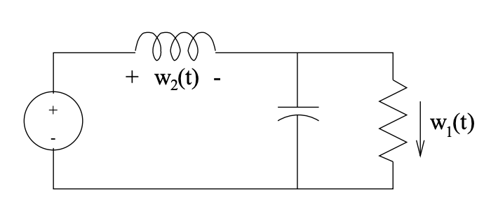
Suppose the signals (variables) of interest - the manifest signals - in the above circuit diagram are \(w_{1}(t)\), \(w_{2}(t)\) and \(w_{3}(t)\) for \(t \geq 0\), so the signal space \(\mathbb{W}\) is \(\mathbb{R}^{3}\) and the time axis \(\mathbb{T}\) is \(\mathbb{R}^{+}\) (i.e. the interval \([0, \infty]\)). Picking all other component voltages and currents as latent signals, we can write the constraints that define the model as:

\[$\left\{\begin{array}{l}2 \text { Kirchhoff's voltage law }(\mathrm{KVL}) \text { equations } \\ 2 \text { Kirchhoff's current law (KCL) equations } \\ 4 \text { defining equations for the components }\end{array}\right.$\nonumber\]

Any set of manifest and latent signals that simultaneously satisfies (or solves) the preceding constraint equations constitutes a behavior, and the behavior \(\mathbb{B}\) of the model is the space of all such solutions.

The same behavior may equivalently be described by a model written entirely in terms of the manifest variables, by eliminating all the other variables in the above equations to obtain

\[0=\frac{w_{1}}{R}+C \dot{w}_{1}-w_{2}\ \tag{6.1}\]

\[0=-w_{3}+L \dot{w}_{2}+w_{1}\ \tag{6.2}\]

Still further reduction to a single second-order differential equation is possible, by taking the derivative of one of these equations and eliminating one variable.

Example 6.2 (Mass- Spring System)

An object of mass \(M\) moves on a horizontal frictionless slide, and is attached to one end of it by a linear spring with spring constant \(k\). A horizontal force \(u(t)\) is applied to the mass. Assume that the variable \(z\) measures the change in the spring length from its natural length. From Newton's law we obtain the model

\[M \ddot{z}=-k z+u\nonumber\]

Example 6.3 (Inverted Pendulum)

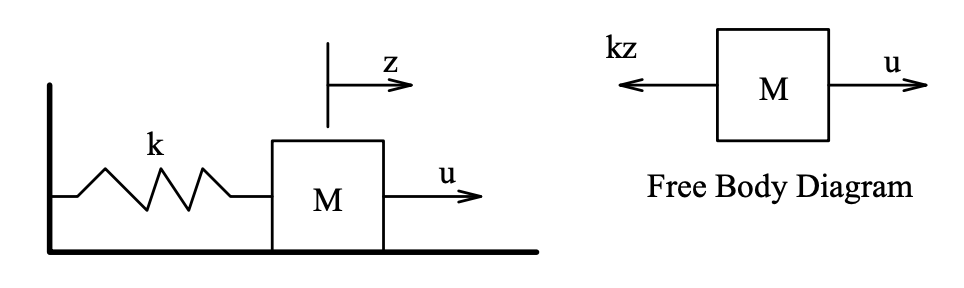
Figure \(\PageIndex{1}\): Mass Spring System.

A cart of mass M slides on a horizontal frictionless track, and is pulled by a horizontal force \(u(t)\). On the cart an inverted pendulum of mass \(m\) is attached via a frictionless hinge, as shown in Figure 28.1. The pendulum's center of mass is located at a distance \(l\) from its two ends, and the pendulum's moment of inertia about its center of mass is denoted by \(I\). The point of support of the pendulum is a distance \(s(t)\) from some reference point. The angle \(\theta(t)\) is the angle that the pendulum makes with respect to the vertical axis. The vertical force exerted by the cart on the base of the pendulum is denoted by \(P\), and the horizontal force by \(N\). What we wish to model are the constraints governing the (manifest) signals \(u(t)\), \(s(t)\) and \(\theta(t)\).

First let us write the equations of motion that result from the free-body diagram of the cart. The vertical forces \(P\), \(R\) and \(Mg\) balance out. For the horizontal forces we have the following equation:

\[M \ddot{s}=u-N\ \tag{6.3}\]

From the free-body diagram of the pendulum, the balance of forces in the hori- zontal direction gives the equation

\[\begin{aligned}
m \frac{d^{2}}{d t^{2}}(s+l \sin (\theta)) &=N, \ or \\
m\left(\ddot{s}-l \sin (\theta)(\dot{\theta})^{2}+l \cos (\theta) \ddot{\theta}\right) &=N, \ (6.4)
\end{aligned} \nonumber\]

and the balance of forces in the vertical direction gives the equation

\[\begin{aligned}
m \frac{d^{2}}{d t^{2}}(l \cos (\theta)) &=P-m g, \ or \\
m\left(-l \cos (\theta)(\dot{\theta})^{2}-l \sin (\theta) \ddot{\theta}\right) &=P-m g. \ (6.5)
\end{aligned} \nonumber\]

From equations (28.16) and (28.17) we can eliminate the force \(N\) to obtain

\[(M+m) \ddot{s}+m\left(l \cos (\theta) \ddot{\theta}-l \sin (\theta)(\dot{\theta})^{2}\right)=u \ \tag{6.6}\]

By balancing the moments around the center of mass, we get the equation

\[I \ddot{\theta}=P l \sin (\theta)-N l \cos (\theta) \ \tag{6.7}\]

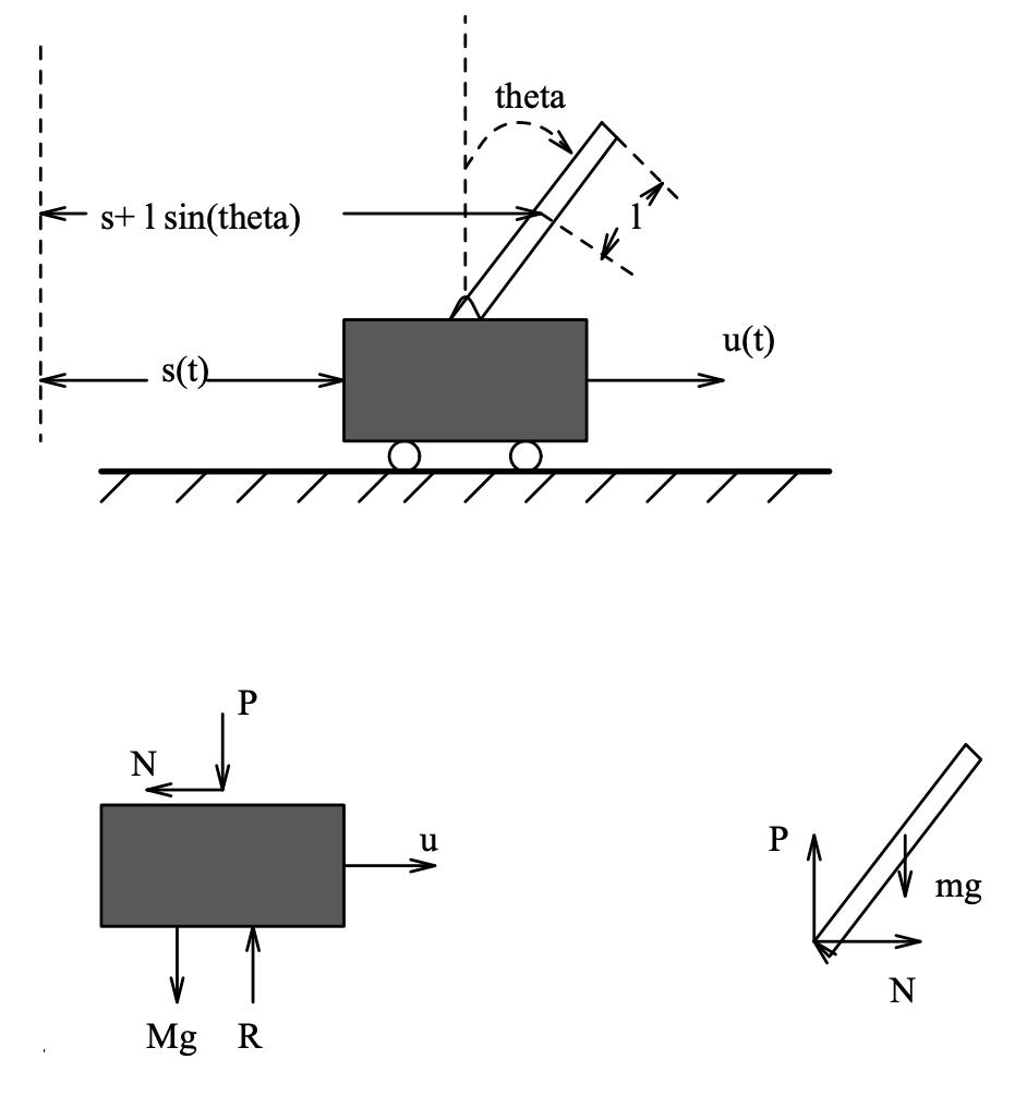
Figure \(\PageIndex{2}\): Inverted Pendulum

Substituting (28.17) and (28.18) into (28.19) gives us

\[\begin{aligned}
I \ddot{\theta} &=l\left(m g-m l \cos (\theta)(\dot{\theta})^{2}-m l \sin (\theta) \ddot{\theta}\right) \sin (\theta) \\
&-l\left(m \ddot{s}-m l \sin (\theta)(\dot{\theta})^{2}+m l \cos (\theta) \ddot{\theta}\right) \cos (\theta)
\end{aligned}\nonumber\]

Simplifying the above expression gives us the equation

\[\left(I+m l^{2}\right) \ddot{\theta}=m g l \sin (\theta)-m l \ddot{s} \cos (\theta)\ \tag{6.8}\]

The equations that comprise our model for the system are (28.20) and (28.21).

We can have a further simplification of the system of equations by removing the term \( \ddot{\theta}\) from equation (28.20), and the term \( \ddot{s}\) from equation (28.21). Define the constants

\[\begin{aligned}
\mathcal{M} &=M+m \\
L &=\frac{I+m l^{2}}{m l}
\end{aligned}\nonumber\]

Substituting \( \ddot{\theta}\) from (28.21) into (28.20), we get

\[\left(1-\frac{m l}{\mathcal{M} L} \cos (\theta)^{2}\right) \ddot{s}+\frac{m l}{\mathcal{M} L} g \sin (\theta) \cos (\theta)-\frac{m l}{\mathcal{M}} \sin (\theta)(\dot{\theta})^{2}=\frac{1}{\mathcal{M}} u \ \tag{6.9}\]

Similarly we can substitute \( \ddot{s}\) from (28.20) into (28.21) to get

\[\left(1-\frac{m l}{\mathcal{M} L} \cos (\theta)^{2}\right) \ddot{\theta}-\frac{g}{L} \sin (\theta)+\frac{m l}{\mathcal{M} L} \sin (\theta) \cos (\theta)(\dot{\theta})^{2}=-\frac{1}{\mathcal{M} L} \cos (\theta) u. \ \tag{6.10}\]

Example 6.4 (Predator-Prey Model)

While the previous examples are physically based, there are many examples of dynamic models that are hypothesized on the basis of a behavioral pattern. For a classical illustration, consider an island populated primarily by goats and foxes. Goats survive on the island's vegetation while foxes survive by eating goats.

To build a model of the population growth of these two interacting animals, define:

\[N_{1}(t)= \text{number of goats at time t} \ \tag{6.11}\]

\[N_{2}(t)= \text{number of foxes at time t} \ \tag{6.12}\]

where \(t\) refers to (discrete) time measured in multiples of months. Volterra proposed the following model:

\[N_{1}(t+1)=a N_{1}(t)-b N_{1}(t) N_{2}(t)\ \tag{6.13}\]

\[N_{2}(t+1)=c N_{2}(t)+d N_{1}(t) N_{2}(t)\ \tag{6.14}\]

The constants \(a\), \(b\), \(c\) and \(d\) are all positive, with \(a > 1\), \(c < 1\). If there were no goats on the island, \(N_{1}(0) = 0\), then - according to this model - the foxes' population would decrease geometrically (i.e. as a discrete-time exponential). If there were no foxes on the island, then the goat population would grow geometrically (presumably there is an unlimited supply of vegetation, water and space). On the other hand, if both species existed on the island, then the frequency of their encounters, which is modeled as being proportional to the product \(N_{1}N_{2}\), determines at what rate goats are eaten and foxes are well-fed. Among the questions that might now be asked are: What sorts of qualitative behavioral characteristics are associated with such a model, and what predictions follow from this behavior? What choices of the parameters \(a\), \(b\), \(c\), \(d\) best match the behavior observed in practice?

Example 6.5 (Smearing in an Imaging System)

Consider a model that describes the relationship between a two-dimensional object and its image on a planar film in a camera. Due to limited aperture, lens imperfections and focusing errors, the image of a unit point source at the origin in the object, represented by the unit impulse \(\delta (x, y)\) in the object plane, will be smeared. The intensity of the light at the image may be modeled by some function \(h(x, y), x, y \in R\), for example \(h(x, y) = e^{-a(x^{2}+y^{2})}\). An object \(u(x, y)\) can be viewed as the superposition of individual points distributed spatially, i.e.,

\[u(x, y)=\iint_{-\infty}^{\infty} \delta(x-\lambda, y-\mu) u(\lambda, \mu) d \lambda d \mu\nonumber\]

Assuming that the effect of the lens is linear and translation invariant, the image of such an object is given by the following intensity function:

\[m(x, y)=\iint_{-\infty}^{\infty} h(x-\lambda, y-\mu) u(\lambda, d \mu) d \lambda d \mu\nonumber\]

We can view u as the input to this system, \(m\) as the output.