
7.2: General Description
- Page ID
- 24270

For a causal system with \(m\) inputs \(u_{j}(t)\) and \(p\) outputs \(y_{i}(t)\) (hence \(m+ p\) manifest variables), an \(n\)th-order state-space description is one that introduces \(n\) latent variables \(x_{l}(t)\) called state variables in order to obtain a particular form for the constraints that define the model. Letting
\[u(t)=\left[\begin{array}{c}
u_{1}(t) \\
\vdots \\
u_{m}(t)
\end{array}\right], \quad y(t)=\left[\begin{array}{c}
y_{1}(t) \\
\vdots \\
y_{p}(t)
\end{array}\right], \quad x(t)=\left[\begin{array}{c}
x_{1}(t) \\
\vdots \\
x_{n}(t)
\end{array}\right]\nonumber\]
an \(n\)th-order state-space description takes the form
\[\underbrace{\dot{x}(t)=f(x(t), u(t), t)}_{\text{state evolution equations}} \label{7.1}\]
\[\underbrace{y(t)=g(x(t), u(t), t)}_{\text{instantaneous output equations}} \label{7.2}\]
To save writing the same equations over for both continuous and discrete time, we interpret
\[\dot{x}(t)=\frac{d x(t)}{d t}, t \in \mathbb{R} \text { or } \mathbb{R}^{+} \nonumber\]
for CT systems, and
\[\dot{x}(t)=x(t+1), \quad t \in \mathbb{Z} \text { or } \mathbb{Z}^{+}\nonumber\]
for DT systems. We will only consider finite-order (or finite-dimensional, or lumped) state-space models, although there is also a rather well developed (but much more subtle and technical) theory of infinite-order (or infinite-dimensional, or distributed) state-space models.
DT Models
The key feature of a state-space description is the following property, which we shall refer to as the state property. Given the present state vector (or "state") and present input at time \(t\), we can compute: (i) the present output, using Equation \ref{7.2}; and (ii) the next state using Equation \ref{7.1}. It is easy to see that this puts us in a position to do the same thing at time \(t + 1\), and therefore to continue the process over any time interval. Extending this argument, we can make the following claim:
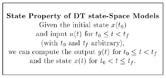
Thus, the state at any time \(t_{0}\) summarizes everything about the past that is relevant to the future. Keeping in mind this fact - that the state variables are the memory variables (or, in more physical situations, the energy storage variables) of a system - often guides us quickly to good choices of state variables in any given context.
CT Models
The same state property turns out to hold in the CT case, at least for \(f ( . )\) that are well behaved enough for the state evolution equations to have a unique solution for all inputs of interest and over the entire time axis | these will typically be the only sorts of CT systems of interest to us. A demonstration of this claim, and an elucidation of the precise conditions under which it holds, would require an excursion into the theory of differential equations beyond what is appropriate for this course. We can make this result plausible, however, by considering the Taylor series approximation
\[\begin{align} x\left(t_{0}+\epsilon\right) &\approx x\left(t_{0}\right)+\left(\frac{d x(t)}{d t}\right)_{t=t_{0}} \epsilon\ \label{7.3} \\[4pt] &=x\left(t_{0}\right)+f\left(x\left(t_{0}\right), u\left(t_{0}\right), t_{0}\right) \epsilon \label{7.4} \end{align}\]
where the second equation results from applying the state evolution Equation \ref{7.1}. This suggests that we can approximately compute \(x(t_{0} + \epsilon)\), given \(x(t_{0})\) and \(u(t_{0})\); the error in the approximation is of order \(\epsilon^{2}\), and can therefore be made smaller by making \(\epsilon\) smaller. For sufficiently well behaved \(f ( . )\), we can similarly step forwards from \(t_{0}+\epsilon \text { to } t_{0}+2 \epsilon\), and so on, eventually arriving at the final time \(t_{f}\), taking on the order of \(\epsilon^{-1}\) steps in the process. The accumulated error at time \(t_{f}\) is then of order \(\epsilon^{-1} \cdot \epsilon^{2}=\epsilon\), and can be made arbitrarily small by making \(\epsilon\) sufficiently small. Also note that, once the state at any time is determined and the input at that time is known, then the output at that time is immediately given by Equation \ref{7.2}, even in the CT case.
The simple-minded Taylor series approximation in Equation \ref{7.4} corresponds to the crudest of numerical schemes - the "forward Euler" method - for integrating a system of equations of the form in Equation \ref{7.1}. Far more sophisticated schemes exist (e.g. Runge-Kutta methods, Adams-Gear schemes for "stiff" systems that exhibit widely differing time scales, etc.), but the forward Euler scheme suffices to make plausible the fact that the state property highlighted above applies to CT systems as well as DT ones.
Example 7.1 RC Circuit
This example demonstrates a fine point in the definition of a state for CT systems. Consider an RC circuit in series with a voltage source \(u\). Using KVL, we get the following equation describing the system:
\[-u+v_{R}+R C \dot{v}_{C}=0\nonumber\]
It is clear that \(v_{C}\) defines a state for the system as we described before. Does \(v_{R}\) define a state? If \(v_{R}(t_{0})\) is given, and the input \(u(t), t_{0} \leq t < t_{f}\) is known, then one can compute \(v_{C}(t_{0})\) and using the state property \(v_{C}(t_{f})\) can be computed from which \(v_{R}(t_{f})\) can be computed. This says that \(v_{R}(t)\) defines a state which contradicts our intuition since it is not an energy storage component.
There is an easy fix of this problem if we assume that all inputs are piece-wise continuous functions. In that case we define the state property as the ability to compute future values of the state from the initial value \(x(t_{0})\) and the input \(u(t), t_{0} < t < t_{f}\). Notice the strict inequality. We leave it to you to verify that this definition rules out \(v_{R}\) as a state variable.
Linearity and Time-Invariance
If in the state-space description in Equation \ref{7.1}, (7.2), we have
\[f(x(t), u(t), t)=f(x(t), u(t))\ \tag{7.5}\]
\[g(x(t), u(t), t)=g(x(t), u(t))\ \tag{7.6}\]
then the model is time-invariant (in the sense defined earlier, for behavioral models). This corresponds to requiring time-invariance of the functions that specify how the state variables and inputs are combined to determine the state evolution and outputs. The results of experiments on a time-invariant system depend only on the inputs and initial state, not on when the experiments are performed.
If, on the other hand, the functions \(f ( . )\) and \(g( . )\) in the state-space description are linear functions of the state variables and inputs, i.e. if
\[f(x(t), u(t), t)=A(t) x(t)+B(t) u(t) \label{7.7}\]
\[g(x(t), u(t), t)=C(t) x(t)+D(t) u(t) \label{7.8}\]
then the model is linear, again in the behavioral sense. The case of a linear and periodically varying (LPV) model is often of interest; when \(A(t) = A(t + T ), B(t) = B(t + T ), C(t) = C(t + T )\), and \(D(t) = D(t + T )\) for all \(t\), the model is LPV with period \(T\).
Of even more importance to us is the case of a model that is linear and time-invariant (LTI). For an LTI model, the state-space description simplifies to
\[f(x(t), u(t), t)=A x(t)+B u(t) \label{7.9} \]
\[g(x(t), u(t), t)=C x(t)+D u(t) \label{7.10}\]
We will primarily study LTI models in this course. Note that LTI state-space models are sometimes designated as \((A, B, C, D)\) or
\[\left[\begin{array}{c|c}
A & B \\
\hline C & D
\end{array}\right]\nonumber\]
as these four matrices completely specify the state-space model.
| System | Type |
|---|---|
| \(\dot{x}(t)=tx^{2}(t)\) | NLTV |
| \(\dot{x}(t)=x^{2}(t)\) | NLTI |
| \(\dot{x}(t)=t x(t)\) | LTV |
| \(\dot{x}(t)=(\cos t) x(t)\) | LPV |
| \(\dot{x}(t)= x(t)\) | LTI |
Some examples of the various classes of systems listed above are given in Table 7.1. More elaborate examples follow.
One might think that the state-space formulation is restrictive since it only involves first-order derivatives. However, by appropriately choosing the state variables, higher-order dynamics can be described. The examples in this section and on homework will make this clear.
Example 7.2: Mass- Spring System
For the mass-spring system in Example 6.2, we derived the following system representation:
\[M \ddot{z}=-k z+u\nonumber\]
To put this in state space form, choose position and velocity as state variables:
\[\begin{array}{l}
x_{1}=z \\
x_{2}=\dot{z} \ (7.11)
\end{array}\nonumber\]
Therefore,
\[\begin{aligned}
\dot{x}_{1} &=\dot{z}=x_{2} \\
\dot{x}_{2} &=-\frac{k}{M} z+\frac{1}{M} u=-\frac{k}{M} x_{1}+\frac{1}{M} u
\end{aligned}\nonumber\]
The input is the force \(u\) and let the output be the position of the mass. The resulting state space description of this system is
\[\left[\begin{array}{c}
\dot{x}_{1} \\
\dot{x}_{2}
\end{array}\right]=\left[\begin{array}{c}
x_{2} \\
-\frac{k}{M} x_{1}+\frac{1}{M} u
\end{array}\right]\nonumber\]
\[\begin{equation}
y=x_{1}
\end{equation}\nonumber\]
The above example suggests something that is true in general for mechanical systems: the natural state variables are the position and velocity variables (associated with potential energy and kinetic energy respective
Example 7.3: Nonlinear Circuit
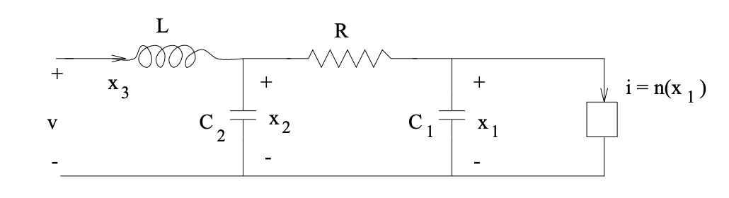
Figure \(\PageIndex{1}\): Nonlinear Circuit
We wish to put the relationships describing the above circuit's behavior in state- space form, taking the voltage \(v\) as an input, and choosing as output variables the voltage across the nonlinear element and the current through the inductor. The constituent relationship for the nonlinear admittance in the circuit diagram is \(i_{nonlin} = \mathcal{N} (v_{nonlin})\), where \(N ( . )\) denotes some nonlinear function.
Let us try taking as our state variables the capacitor voltages and inductor current, because these variables represent the energy storage mechanisms in the circuit. The corresponding state-space description will express the rates of change of these variables in terms of the instantaneous values of these variables and the instantaneous value of the input voltage \(v\). It is natural, therefore, to look for expressions for \(C_{1} \dot{x}_{1}\) (the current through \(C_{1}\), for \(C_{2} \dot{x}_{2}\) (the current through \(C_{2}\), and for \(L \dot{x}_{3}\) (the voltage across \(L\)).
Applying KCL to the node where \(R\), \(C_{1}\), and the nonlinear device meet, we get
\[C_{1} \dot{x}_{1}=\frac{\left(x_{2}-x_{1}\right)}{R}-\mathcal{N}\left(x_{1}\right)\nonumber\]
Applying KCL to the node where \(R\), \(C_{2}\) and \(L\) meet, we find
\[C_{2} \dot{x}_{2}=x_{3}-\frac{\left(x_{2}-x_{1}\right)}{R}\nonumber\]
Finally, KVL applied to a loop containing \(L\) yields
\[L \dot{x}_{3}=v-x_{2}\nonumber\]
Now we can combine these three equations to obtain a state-space description of this system:
\[\left[\begin{array}{c}
\dot{x}_{1} \\
\dot{x}_{2} \\
\dot{x}_{3}
\end{array}\right]=\left[\begin{array}{c}
\frac{1}{C_{1}}\left(\frac{x_{2}-x_{1}}{R}-\mathcal{N}\left(x_{1}\right)\right) \\
\frac{1}{C_{2}}\left(x_{3}-\frac{x_{2}-x_{1}}{R}\right) \\
-\frac{1}{L} x_{2}
\end{array}\right]+\left[\begin{array}{c}
0 \\
0 \\
\frac{1}{L} v
\end{array}\right] \ \tag{7.12}\]
\[y=\left[\begin{array}{l}
x_{1} \\
x_{3}
\end{array}\right]\ \tag{7.13}\]
Observe that the output variables are described by an instantaneous output equation of the form (7.2). This state-space description is time-invariant but nonlinear. This makes sense, because the circuit does contain a nonlinear element!
Example 7.4: Discretization
Assume we have a continuous-time system described in state-space form by
\[\begin{aligned}
\frac{d x(t)}{d t} &=A x(t)+B u(t) \\
y(t) &=C x(t)+D u(t)
\end{aligned}\nonumber\]
Let us now sample this system with a period of \(T\), and approximate the derivative as a forward difference:
\[\frac{1}{T}(x((k+1) T)-x(k T))=A x(k T)+B u(k T), \quad k \in \mathbb{Z} \label{7.14}\]
It is convenient to change our notation, writing \(x[k] \equiv x(k T)\), and similarly for \(u\) and \(y\). Our sampled equation can thereby be rewritten as
\[\begin{aligned}
x[k+1] &=(I+T A) x[k]+T B u[k] \\
&=\hat{A} \mathbf{x}[k]+\hat{B} \mathbf{u}[k] \\
y[k] &=C x[k]+D u[k] \ (7.15)
\end{aligned}\nonumber\]
which is in standard state-space form.
In many modern applications, control systems are implemented digitally. For that purpose, the control engineer must be able to analyze both discrete-time as well as continuous-time systems. In this example a crude sampling method was used to obtain a discrete-time model from a continuous-time one. We will discuss more refined discretization methods later on in this book.
It is also important to point out that there are physical phenomena that directly require or suggest discrete-time models; not all discrete-time models that one encounters in applications are discretizations of continuous-time ones.