8.2: Realization from I/O Representations

In this section, we will describe how a state space realization can be obtained for a causal input-output dynamic system described in terms of convolution.

8.2.1 Convolution with an Exponential

Consider a causal DT LTI system with impulse response \(h[n]\) (which is 0 for \(n < 0\)):

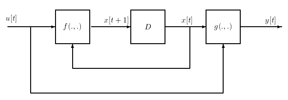
Figure \(\PageIndex{1}\): Simulation Diagram

\[\begin{aligned}
y[n] &=\sum_{-\infty}^{n} h[n-k] u[k] \\
&=\left(\sum_{-\infty}^{n-1} h[n-k] u[k]\right)+h[0] u[n]
\end{aligned} \ \tag{8.3}\]

The first term above, namely

\[x[n]=\sum_{-\infty}^{n-1} h[n-k] u[k]\ \tag{8.4}\]

represents the effect of the past on the present. This expression shows that, in general (i.e. if \(h[n]\) has no special form), the number \(x[n]\) has to be recomputed from scratch for each \(n\). When we move from \(n\) to \(n + 1\), none of the past input, i.e. \(u[k]\) for \(k \leq n\), can be discarded, because all of the past will again be needed to compute \(x[n + 1]\). In other words, the memory of the system is infinite.

Now look at an instance where special structure in \(h[n]\) makes the situation much better.

Suppose

\[h[n]=\lambda^{n} \text{ for } n \geq 0,\text{and 0 otherwise}\ \tag{8.5}\]

Then

\[x[n]=\sum_{-\infty}^{n-1} \lambda^{n-k} u[k] \ \tag{8.6}\]

and

\[\begin{aligned}
x[n+1] &=\sum_{-\infty}^{n} \lambda^{n+1-k} u[k] \\
&=\lambda\left(\sum_{-\infty}^{n-1} \lambda^{n-k} u[k]\right)+\lambda u[n] \\
&=\lambda x[n]+\lambda u[n]
\end{aligned} \ \tag{8.7}\]

(You will find it instructive to graphically represent the convolutions that are involved here, in order to understand more visually why the relationship (8.7) holds.) Gathering (8.3) and (8.6) with (8.7), we obtain a pair of equations that together constitute a state-space description for this system:

\[x[n+1]=\lambda x[n]+\lambda u[n] \ \tag{8.8}\]

\[y[n=x[n]+ u[n] \ \tag{8.9}\]

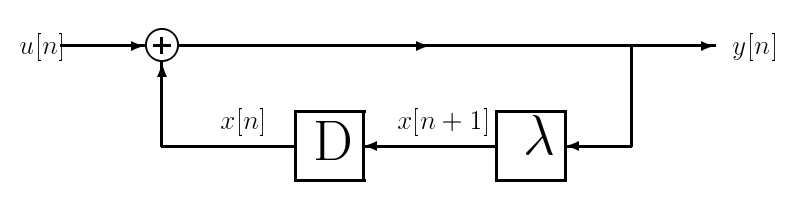
To realize this model in hardware, or to simulate it, we can use a delay-adder-gain system that is obtained as follows. We start with a delay element, whose output will be \(x[n]\) when its input is \(x[n+1]\). Now the state evolution equation tells us how to combine the present output of the delay element, \(x[n]\), with the present input to the system, \(u[n]\), in order to obtain the present input to the delay element, \(x[n + 1]\). This leads to the following block diagram, in which we have used the output equation to determine how to obtain \(y[n]\) from the present state and input of the system:

8.2.2 Convolution with a Sum of Exponentials

Consider a more complicated causal impulse response than the previous example, namely

\[h[n]=\rho_{0} \delta[n]+\left(\rho_{1} \lambda_{1}^{n}+\rho_{2} \lambda_{2}^{n}+\cdots+\rho_{L} \lambda_{L}^{n}\right) \ \tag{8.10}\]

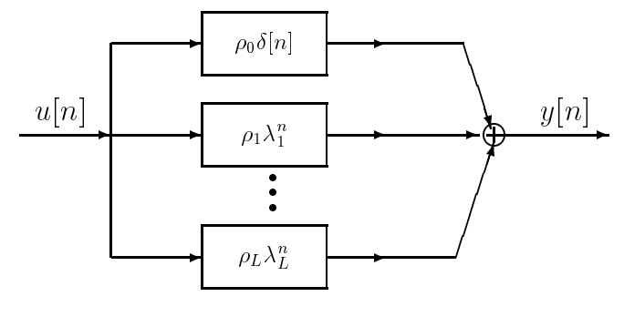
with the \(\rho_{i}\) being constants. The following block diagram shows that this system can be considered as being obtained through the parallel interconnection of causal subsystems that are as simple as the one treated earlier, plus a direct feedthrough of the input through the gain \(\rho_{0}\) (each block is labeled with its impulse response, with causality implying that these responses are 0 for \(n < 0\)):

Motivated by the above structure and the treatment of the earlier, let us define a state variable for each of the \(L\) subsystems:

\[x_{i}[n]=\sum_{-\infty}^{n-1} \lambda_{i}^{n-k} u[k], \quad i=1,2, \ldots, L \ \tag{8.11}\]

With this, we immediately obtain the following state-evolution equations for the subsystems:

\[x_{i}[n+1]=\lambda_{i} x_{i}[n]+\lambda_{i} u[n], \quad i=1,2, \ldots, L \ \tag{8.12}\]

Also, after a little algebra, we directly find

\[y[n]=\rho_{1} x_{1}[n]+\rho_{2} x_{2}[n]+\cdots+\rho_{L} x_{L}[n]+\left(\sum_{0}^{L} \rho_{i}\right) u[n] \ \tag{8.13}\]

We have thus arrived at an \(L\)th-order state-space description of the given system. To write the above state-space description in matrix form, define the state vector at time \(n\) to be

\[\mathbf{x}[n]=\left(\begin{array}{c}
x_{1}[n] \\
x_{2}[n] \\
\vdots \\
x_{L}[n]
\end{array}\right) \ \tag{8.14}\]

Also define the diagonal matrix \(\mathbf{A}\), column vector \(\mathbf{b}\), and row vector \(\mathbf{c}\) as follows:

\[\mathbf{A}=\left(\begin{array}{cccccc}
\lambda_{1} & 0 & 0 & \cdots & 0 & 0 \\
0 & \lambda_{2} & 0 & \cdots & 0 & 0 \\
\vdots & \vdots & \vdots & \ddots & \vdots & \vdots \\
0 & 0 & 0 & \cdots & 0 & \lambda_{L}
\end{array}\right), \quad \mathbf{b}=\left(\begin{array}{c}
\lambda_{1} \\
\lambda_{2} \\
\vdots \\
\lambda_{L}
\end{array}\right) \ \tag{8.15}\]

\[\mathbf{c}=\left(\begin{array}{cccccc}
\rho_{1} & \rho_{2} & \cdots & \cdots & \cdots & \rho_{L}
\end{array}\right) \ \tag{8.16}\]

Then our state-space model takes the desired matrix form, as you can easily verify:

\[\begin{aligned}
\mathrm{x}[n+1] &=\mathbf{A} \mathbf{x}[n]+\mathbf{b} u[n] \ (8.17)\\
y[n] &=\mathbf{c x}[n]+\mathrm{d} u[n] \ (8.18)
\end{aligned}\nonumber\]

where

\[\mathrm{d}=\sum_{0}^{L} \rho_{i}\ \tag{8.19}\]