8.3: Realization from an LTI Differential/ Difference equation

In this section, we describe how a realization can be obtained from a difference or a differential equation. We begin with an example.

Example 8.1 (State-Space Models for an LTI Difference Equation)

Let us examine some ways of representing the following input-output difference equation in state-space form:

\[y[n]+a_{1} y[n-1]+a_{2} y[n-2]=b_{1} u[n-1]+b_{2} u[n-2]\ \tag{8.20}\]

For a first attempt, consider using as state vector the quantity

\[\mathbf{x}[n]=\left(\begin{array}{c}
y[n-1] \\
y[n-2] \\
u[n-1] \\
u[n-2]
\end{array}\right) \ \tag{8.21}\]

The corresponding 4th-order state-space model would take the form

\[\mathbf{x}[n+1]=\left(\begin{array}{c}
y[n] \\
y[n-1] \\
u[n] \\
u[n-1]
\end{array}\right)=\left(\begin{array}{cccc}
-a_{1} & -a_{2} & b_{1} & b_{2} \\
1 & 0 & 0 & 0 \\
0 & 0 & 0 & 0 \\
0 & 0 & 1 & 0
\end{array}\right)\left(\begin{array}{l}
y[n-1] \\
y[n-2] \\
u[n-1] \\
u[n-2]
\end{array}\right)+\left(\begin{array}{c}
0 \\
0 \\
1 \\
0
\end{array}\right) u[n]\nonumber\]

\[y[n]=\left(\begin{array}{cccc}
-a_{1} & -a_{2} & b_{1} & b_{2}
\end{array}\right)\left(\begin{array}{c}
y[n-1] \\
y\left[\begin{array}{c}
n-2
\end{array}\right] \\
u[n-1] \\
u[n-2]
\end{array}\right)+\left(\begin{array}{l}
0 \\
u[n-1]
\end{array}\right) u\left[n\right]\ \tag{8.22}\]

If we are somewhat more careful about our choice of state variables, it is possible to get more economical models. For a 3rd-order model, suppose we pick as state vector

\[\mathbf{x}[n]=\left(\begin{array}{c}
y[n] \\
y[n-1] \\
u[n-1]
\end{array}\right) \ \tag{8.23}\]

The corresponding 3rd-order state-space model takes the form

\[\mathbf{x}[n+1]=\left(\begin{array}{c}
y[n+1] \\
y[n] \\
u[n]
\end{array}\right)=\left(\begin{array}{ccc}
-a_{1} & -a_{2} & b_{2} \\
1 & 0 & 0 \\
0 & 0 & 0
\end{array}\right)\left(\begin{array}{c}
y[n] \\
y[n-1] \\
u[n-1]
\end{array}\right)+\left(\begin{array}{c}
b_{1} \\
0 \\
1
\end{array}\right) u[n]\nonumber\]

\[y[n]=\left(\begin{array}{ccc}
1 & 0 & 0
\end{array}\right)\left(\begin{array}{c}
y[n] \\
y[n-1] \\
u[n-1]
\end{array}\right)+\left(\begin{array}{l}
0
\end{array}\right) u[n] \ \tag{8.24}\]

A still more clever/devious choice of state variables yields a 2nd-order state-space model. For this, pick

\[\mathbf{x}[n]=\left(\begin{array}{c}
y[n] \\
-a_{2} y[n-1]+b_{2} u[n-1]
\end{array}\right)\ \tag{8.25}\]

The corresponding 2nd-order state-space model takes the form

\[\begin{aligned}
\left(\begin{array}{c}
y[n+1] \\
-a_{2} y[n]+b_{2} u[n]
\end{array}\right) &=\left(\begin{array}{cc}
-a_{1} & 1 \\
-a_{2} & 0
\end{array}\right)\left(\begin{array}{c}
y[n] \\
-a_{2} y[n-1]+b_{2} u[n-1]
\end{array}\right)+\left(\begin{array}{c}
b_{1} \\
b_{2}
\end{array}\right) u[n] \\
y[n] &=\left(\begin{array}{cc}
1 & 0
\end{array}\right)\left(\begin{array}{c}
y[n] \\
-a_{2} y[n-1]+b_{2} u[n-1]
\end{array}\right)+\left(\begin{array}{c}
0
\end{array}\right) u[n]
\end{aligned} \ \tag{8.26}\]

It turns out to be impossible in general to get a state-space description of order lower than 2 in this case. This should not be surprising, in view of the fact that we started with a 2nd-order difference equation, which we know (from earlier courses!) requires two initial conditions in order to solve forwards in time. Notice how, in each of the above cases, we have incorporated the information contained in the original difference equation that we started with.

This example was built around a second-order difference equation, but has natural generalizations to the \(n\)th-order case, and natural parallels in the case of CT differential equations.

Next, we will present two realizations of an \(n\)th-Order LTI differential equation. While realizations are not unique, these two have certain nice properties that will be discussed in the future.

8.3.1 Observability Canonical Form

Suppose we are given the LTI differential equation

\[y^{(n)}+a_{n-1} y^{(n-1)}+\cdots+a_{0} y=b_{0} u+b_{1} \dot{u}+\cdots+b_{n-1} u^{(n-1)}\nonumber\]

which can be rearranged as

\[y^{(n)}=\left(b_{n-1} u^{(n-1)}-b_{n-1} y^{(n-1)}\right)+\left(b_{n-2} u^{(n-2)}-a_{n-2} y^{(n-2)}\right)+\cdots+\left(b_{0} u-a_{0} y\right)\nonumber\]

Integrated \(n\) times, this becomes

\[y=\int\left(b_{n-1} u-a_{n-1} y\right)+\iint\left(b_{n-2} u-a_{n-2} y\right)+\cdots+\int \ldots \int\left(b_{0} u-a_{0} y\right)\ \tag{8.27}\]

The block diagram given in Figure 8.3.1 then follows directly from (8.27). This particular realization is called the observability canonical form realization -"canonical" in the sense of

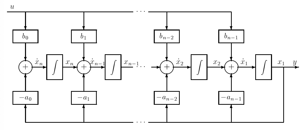
Figure \(\PageIndex{1}\): Observability Canonical Form

"simple" (but there is actually a strict mathematical definition as well), and "observability" for reasons that will emerge later in the course.

We can now read the state equations directly from Figure 8.3.1, once we recognize that the natural state variables are the outputs of the integrators:

\[\begin{aligned}
\dot{x}_{1} &=-a_{n-1} x_{1}+x_{2}+b_{n-1} u \\
\dot{x}_{2} &=-a_{n-2} x_{1}+x_{3}+b_{n-2} u \\
& \vdots \\
\dot{x}_{n} &=-a_{0} x_{1}+b_{0} u \\
y &=x_{1}
\end{aligned}\nonumber\]

If this is written in our usual matrix form, we would have

\[A=\left[\begin{array}{ccccc}
-a_{n-1} & 1 & 0 & \cdots & 0 \\
-a_{n-2} & 0 & 1 & \cdots & 0 \\
\vdots & & & \ddots & \\
& & & & 1 \\
-a_{0} & 0 & & \cdots & 0
\end{array}\right],
\ b\left[\begin{array}{c}
b_{n-1} \\
b_{n-2} \\
\vdots \\
\vdots \\
b_{0}
\end{array}\right]\nonumber\]

\[c=\left[\begin{array}{llll}
1 & 0 & \cdots & 0
\end{array}\right]\nonumber\]

The matrix \(A\) is said to be in companion form, a term used to refer to any one of four matrices whose pattern of 0's and 1's is, or resembles, the pattern seen above. The characteristic polynomial of such a matrix can be directly read off from the remaining coefficients, as we shall see when we talk about these polynomials, so this matrix is a "companion" to its characteristic polynomial.

8.3.2 Reachability Canonical Form

There is a "dual" realization to the one presented in the previous section for the LTI differential equation

\[y^{(n)}+a_{n-1} y^{(n-1)}+\cdots+a_{0} y=c_{0} u+c_{1} \dot{u}+\cdots+c_{n-1} u^{(n-1)} \ \tag{8.28}\]

First, consider a special case of this, namely the differential equation

\[w^{(n)}+a_{n-1} w^{(n-1)}+\cdots+a_{0} w=u \ \tag{8.29}\]

To obtain an \(n\)th-order state-space realization of the system in 8.29, define

\[x=\left[\begin{array}{c}
x_{1} \\
x_{2} \\
x_{3} \\
\vdots \\
x_{n-1} \\
x_{n}
\end{array}\right]=\left[\begin{array}{c}
w \\
\dot{w} \\
\ddot{w} \\
\vdots \\
\frac{d^{n-2} w}{d t^{n-2}} \\
\frac{d^{n-1} w}{d t^{n-1}}
\end{array}\right]\nonumber\]

Then it is easy to verify that the following state-space description represents the given model:

\[\frac{d}{dx}\left[\begin{array}{c}
x_{1} \\
x_{2} \\
x_{3} \\
\vdots \\
x_{n-1} \\
x_{n}
\end{array}\right]=
\left[\begin{array}{cccccc}
0 & 1 & 0 & 0 & \cdots & 0 \\
0 & 0 & 1 & 0 & \ldots & 0 \\
0 & 0 & 0 & 1 & \ldots & 0 \\
\vdots & & & & \vdots & \\
0 & 0 & 0 & \ldots & 0 & 1 \\
-a_{0}(t) & -a_{1}(t) & -a_{2}(t) & \ldots & -a_{n-2}(t) & -a_{n-1}(t)
\end{array}\right]
\left[\begin{array}{c}
x_{1} \\
x_{2} \\
x_{3} \\
\vdots \\
x_{n-1} \\
x_{n}
\end{array}\right]+
\left[\begin{array}{c}
0 \\
0 \\
0 \\
\vdots \\
0 \\
1
\end{array}\right]u\nonumber\]

\[w=\left[\begin{array}{cccccc}
w & = & 1 & 0 & 0 & 0 & \ldots & 0
\end{array}\right]\left[\begin{array}{c}
x_{1} \\
x_{2} \\
x_{3} \\
\vdots \\
x_{n-1} \\
x_{n}
\end{array}\right]\nonumber\]

(The matrix A here is again in one of the companion forms; the two remaining companion forms are the transposes of the one here and the transpose of the one in the previous section.)

Suppose now that we want to realize another special case, namely the differential equation

\[r^{(n)}+a_{n-1} r^{(n-1)}+\cdots+a_{0} r=\dot{u}\ \tag{8.30}\]

which is the same equation as (8.29), except that the RHS is \(\dot{u}\) rather than \(u\). By linearity, the response of (8.30) will \(r = \dot{w}(t)\), and this response can be obtained from the above realization by simply taking the output to be \(x_{2}\) rather than \(x_{1}\), since \(x_{2} = \dot{w} = r\).

Superposing special cases of the preceding form, we see that if we have the differential equation (8.28), with an RHS of

\[c_{0} u+c_{1} \dot{u}+\cdots+c_{n-1} u^{(n-1)}\nonumber\]

then the above realization suffices, provided we take the output to be

\[y=c_{0} x_{1}+c_{1} x_{2}+\cdots+c_{n-1} x_{n}\ \tag{8.31}\]

i.e., we just change the output equation to have

\[c=\left[\begin{array}{lllll}
c_{0} & c_{1} & c_{2} & \cdots & c_{n-1}
\end{array}\right]\ \tag{8.32}\]

A block diagram of the final realization is shown below in 8.3.2. This is called the reachability or controllability canonical form.

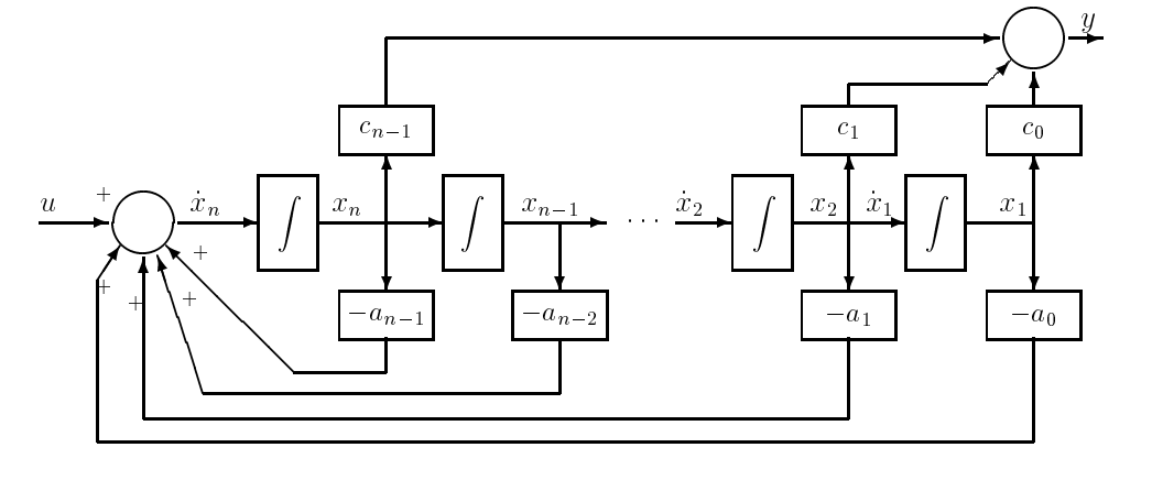
Figure \(\PageIndex{2}\): Reachability Canonical Form

Finally, for the obvious DT difference equation that is analogous to the CT differential equation that we used in this example, the same scheme will work, with derivatives replaced by differences.