13.1: Notions of Stability

For a general undriven system

\[\begin{align} \dot{x}(t) &=f(x(t), 0, t) \quad(C T) \label{13.1}\\[4pt] x(k+1) &=f(x(k), 0, k) \quad(D T) \label{13.2} \end{align}\]

we say that a point \(\bar{x}\) is an equilibrium point from time \(t_{0}\) for the CT system above if \(f(\bar{x}, 0, t)= 0, \forall t \geq t_{0}\), and is an equilibrium point from time \(k_{0}\) for the DT system above if \(f(\bar{x}, 0, k)= \bar{x}, \forall k \geq k_{0}\). If the system is started in the state \(\bar{x}\) at time \(t_{0}\) or \(k_{0}\), it will remain there for all time. Nonlinear systems can have multiple equilibrium points (or equilibria). (Another class of special solutions for nonlinear systems are periodic solutions, but we shall just focus on equilibria here.) We would like to characterize the stability of the equilibria in some fashion. For example, does the state tend to return to the equilibrium point after a small perturbation away from it? Does it remain close to the equilibrium point in some sense? Does it diverge?

The most fruitful notion of stability for an equilibrium point of a nonlinear system is given by the definition below. We shall assume that the equilibrium point of interest is at the origin, since if \(\bar{x} \neq 0\), a simple translation can always be applied to obtain an equivalent system with the equilibrium at 0.

Definition \(\PageIndex{1}\): Asymptotically Stable

A system is called asymptotically stable around its equilibrium point at the origin if it satisfies the following two conditions:

1. Given any \(\epsilon>0, \exists \delta_{1}>0\) such that if \(\left\|x\left(t_{0}\right)\right\|<\delta_{1}\), then \(\|x(t)\|<\epsilon, \forall t>t_{0}\).
2. \(\exists \delta_{2}>0\) such that if \(\left\|x\left(t_{0}\right)\right\|<\delta_{2}\), then \(x(t) \rightarrow 0\) as \(t \rightarrow \infty\).

The first condition requires that the state trajectory can be confined to an arbitrarily small "ball" centered at the equilibrium point and of radius \(\epsilon\), when released from an arbitrary initial condition in a ball of sufficiently small (but positive) radius \(\delta_{1}\). This is called stability in the sense of Lyapunov (i.s.L.). It is possible to have stability in the sense of Lyapunov without having asymptotic stability, in which case we refer to the equilibrium point as marginally stable. Nonlinear systems also exist that satisfy the second requirement without being stable i.s.L., as the following example shows. An equilibrium point that is not stable i.s.L. is termed unstable

Example \(\PageIndex{1}\): Unstable Equilibrium Point That Attracts All Trajectories

Consider the second-order system with state variables \(x_{1}\) and \(x_{2}\) whose dynamics are most easily described in polar coordinates via the equations

\[\begin{align}
\dot{r} &=r(1-r) \\[4pt]
\dot{\theta} &=\sin ^{2}(\theta / 2) \label{13.3}
\end{align}\]

where the radius \(r\) is given by \(r=\sqrt{x_{1}^{2}+x_{2}^{2}}\) and the angle \(\theta\) by \(0 \leq \theta= \arctan \left(x_{2} / x_{1}\right)<2 \pi\). (You might try obtaining a state-space description directly involving \(x_{1}\) and \(x_{2}\).) It is easy to see that there are precisely two equilibrium points: one at the origin, and the other at \(r = 1, \theta = 0\). We leave you to verify with rough calculations (or computer simulation from various initial conditions) that the trajectories of the system have the form shown in the figure below.

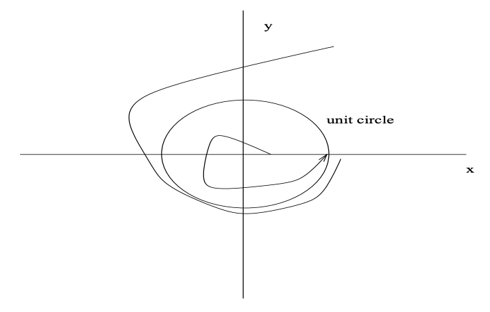
Figure \(\PageIndex{1}\): System Trajectories

Evidently all trajectories (except the trivial one that starts and stays at the origin) end up at \(r = 1, \theta = 0\). However, this equilibrium point is not stable i.s.L., because these trajectories cannot be confined to an arbitrarily small ball around the equilibrium point when they are released from arbitrary points with any ball (no matter how small) around this equilibrium.