13.3: Lyapunov's Direct Method

General Idea

Consider the continuous-time system

\[\dot{x}(t)=f(x(t)) \ \tag{13.8}\]

with an equilibrium point at \(x = 0\). This is a time-invariant (or "autonomous") system, since \(f\) does not depend explicitly on \(t\). The stability analysis of the equilibrium point in such a system is a difficult task in general. This is due to the fact that we cannot write a simple formula relating the trajectory to the initial state. The idea behind Lyapunov's "direct" method is to establish properties of the equilibrium point (or, more generally, of the nonlinear system) by studying how certain carefully selected scalar functions of the state evolve as the system state evolves. (The term "direct" is to contrast this approach with Lyapunov's "indirect" method, which attempts to establish properties of the equilibrium point by studying the behavior of the linearized system at that point. We shall study this next Chapter.)

Consider, for instance, a continuous scalar function \(V (x)\) that is 0 at the origin and positive elsewhere in some ball enclosing the origin, i.e. \(V (0) = 0\) and \(V (x) > 0\) for \(x \neq 0\) in this ball. Such a \(V (x)\) may be thought of as an "energy" function. Let \(\dot{V} (x)\) denote the time derivative of \(V (x)\) along any trajectory of the system, i.e. its rate of change as \(x(t)\) varies according to (13.8). If this derivative is negative throughout the region (except at the origin), then this implies that the energy is strictly decreasing over time. In this case, because the energy is lower bounded by 0, the energy must go to 0, which implies that all trajectories converge to the zero state. We will formalize this idea in the following sections.

Lyapunov Functions

Definition 13.2

Let \(V\) be a continuous map from \(\mathbb{R}^{n}\) to \(\mathbb{R}\). We call \(V (x)\) a locally positive definite (lpd) function around \(x = 0\) if

1. \(V(0)=0\)
2. \(V(x)>0,0<\|x\|<r\) for some \(r\).

Similarly, the function is called locally positive semidefinite (lpsd) if the strict inequality on the function in the second condition is replaced by \(V(x) \geq 0\). The function \(V (x)\) is locally negative definite (lnd) if \(-V (x)\) is lpd, and locally negative semidefinite (lnsd) if \(-V (x)\) is lpsd. What may be useful in forming a mental picture of an lpd function \(V (x)\) is to think of it as having "contours" of constant \(V\) that form (at least in a small region around the origin) a nested set of closed surfaces surrounding the origin. The situation for \(n = 2\) is illustrated in Figure 13.2.

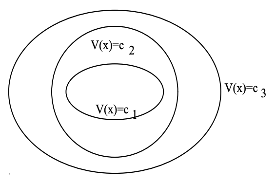
Figure \(\PageIndex{1}\): Level lines for a Lyapunov function, where \(c_{1} < c_{2} < c_{3}\)

Throughout our treatment of the CT case, we shall restrict ourselves to \(V (x)\) that have continuous first partial derivatives. (Differentiability will not be needed in the DT case - continuity will suffice there.) We shall denote the derivative of such a \(V\) with respect to time along a trajectory of the system (13.8) by \(\dot{V} (x(t))\). This derivative is given by

\[\dot{V}(x(t))=\frac{d V(x)}{d x} \dot{x}=\frac{d V(x)}{d x} f\tag{x}\]

where \(\frac{d V(x)}{d x}\) is a row vector - the gradient vector or Jacobian of \(V\) with respect to \(x\) - containing the component-wise partial derivatives \(\frac{\partial V}{\partial x_{i}}\).

Definition 13.3

Let \(V\) be an lpd function (a "candidate Lyapunov function"), and let \(\dot{V}\) be its derivative along trajectories of system (13.8). If \(\dot{V}\) is lnsd, then \(V\) is called a Lyapunov function of the system (13.8).

Lyapunov Theorem for Local Stability

Theorem 13.1

If there exists a Lyapunov function of system (13.8), then \(x = 0\) is a stable equilibrium point in the sense of Lyapunov. If in addition \(\dot{V}(x)<0,0<\|x\|<r_{1}\) for some \(r_{1}\), i.e. if \(\dot{V}\) is lnd, then \(x = 0\) is an asymptotically stable equilibrium point.

Proof

First, we prove stability in the sense of Lyapunov. Suppose \(\epsilon>0\) is given. We need to find a \(\delta>0\) such that for all \(\|x(0)\|<\delta\), it follows that \(\|x(t)\|<\epsilon, \forall t>0\). The Figure 19.6 illustrates the constructions of the proof for the case \(n = 2\). Let \(\epsilon_{1}=\min (\epsilon, r)\). Define

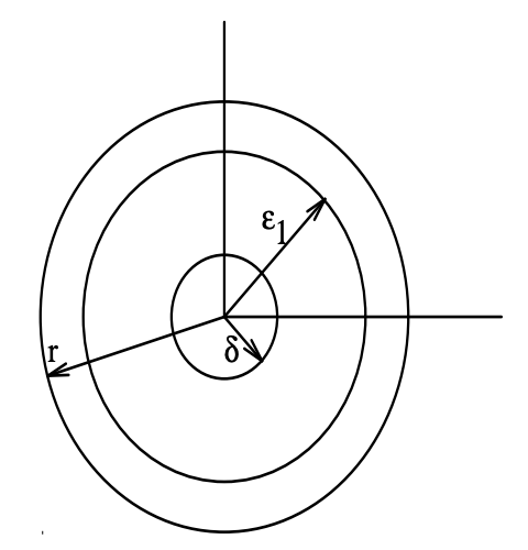
Figure \(\PageIndex{2}\): Illustration of the neighbourhoods used in the proof

\[m=\min _{\|x\|=\epsilon_{1}} V\tag{x}\]

Since \(V (x)\) is continuous, the above \(m\) is well defined and positive. Choose \(\delta\) satisfying \(0<\delta<\epsilon_{1}\) such that for all \(\|x\|<\delta, V(x)<m\). Such a choice is always possible, again because of the continuity of \(V (x)\). Now, consider any \(x(0)\) such that \(\|x(0)\|<\delta, V(x(0))<m\), and let \(x(t)\) be the resulting trajectory. \(V (x(t))\) is non-increasing (i.e. \(\dot{V}(x(t)) \leq 0)\)) which results in \(V (x(t)) < m\). We will show that this implies that \(\|x(t)\|<\epsilon_{1}\). Suppose there exists \(t_{1}\) such that \(\left\|x\left(t_{1}\right)\right\|>\epsilon_{1}\), then by continuity we must have that at an earlier time \(t_{2}\), \(\left\|x\left(t_{2}\right)\right\|=\epsilon_{1}\), and \(\min _{\|x\|=\epsilon_{1}}\|V(x)\|=m>V\left(x\left(t_{2}\right)\right)\), which is a contradiction. Thus stability in the sense of Lyapunov holds.

To prove asymptotic stability when \(\dot{V}\) is lnd, we need to show that as \(t \rightarrow \infty, V(x(t)) \rightarrow 0\) then, by continuity of \(V,\|x(t)\| \rightarrow 0\). Since \(V (x(t))\) is strictly decreasing, and \(V(x(t)) \geq 0\) we know that \(V(x(t)) \rightarrow c\), with \(c \geq 0\). We want to show that \(c\) is in fact zero. We can argue by contradiction and suppose that \(c > 0\). Let the set \(S\) be defined as

\[S=\left\{x \in \mathbb{R}^{n} \mid V(x) \leq c\right\}\nonumber\]

and let \(B_{\alpha}\) be a ball inside \(S\) of radius \(\alpha\),

\[B_{\alpha}=\{x \in S \mid\|x\|<\alpha\}\nonumber\]

Suppose \(x(t)\) is a trajectory of the system that starts at \(x(0)\), we know that \(V (x(t))\) is decreasing monotonically to \(c\) and \(V(x(t))>c\) for all \(t\). Therefore, \(x(t) \notin B_{\alpha}\); recall that \(B_{\alpha} \subset S\) which is defined as all the elements in \(\mathbb{R}^{n}\) for which \(V(x) \leq c\). In the first part of the proof, we have established that if \(\|x(0)\|<\delta\) then \(\|x(t)\|<\epsilon\). We can define the largest derivative of \(V (x)\) as

\[-\gamma=\max _{\alpha \leq\|x\| \leq \epsilon} \dot{V}\tag{x}\]

Clearly \(-\gamma<0\) since \(\dot{V} (x)\) is lnd. Observe that,

\[\begin{aligned}
V(x(t)&=V(x(0))+\int_{0}^{t} \dot{V}(x(\tau)) d \tau \\
& \leq V(x(0))-\gamma t
\end{aligned}\nonumber\]

which implies that \(V (x(t))\) will be negative which will result in a contradiction establishing the fact that \(c\) must be zero.

Example 13.2

Consider the dynamical system which is governed by the differential equation

\[\dot{x}=-g\tag{x}\]

where \(g(x)\) has the form given in Figure 13.4. Clearly the origin is an equilibrium point. If we define a function

\[V(x)=\int_{0}^{x} g(y) d y\nonumber\]

then it is clear that \(V (x)\) is locally positive definite (lpd) and

\[\dot{V}(x)=-g(x)^{2}\nonumber\]

which is locally negative definite (lnd). This implies that \(x = 0\) is an asymptotically stable equilibrium point.

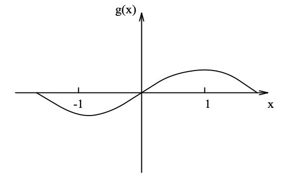
Figure \(\PageIndex{3}\): Graphical Description of g(x)

Lyapunov Theorem for Global Asymptotic Stability

The region in the state space for which our earlier results hold is determined by the region over which \(V (x)\) serves as a Lyapunov function. It is of special interest to determine the "basin of attraction" of an asymptotically stable equilibrium point, i.e. the set of initial conditions whose subsequent trajectories end up at this equilibrium point. An equilibrium point is globally asymptotically stable (or asymptotically stable "in the large") if its basin of attraction is the entire state space.

If a function \(V (x)\) is positive definite on the entire state space, and has the additional property that \(|V(x)| \nearrow \infty\) as \(\|x\| \nearrow \infty\), and if its derivative \(V\) is negative definite on the entire state space, then the equilibrium point at the origin is globally asymptotically stable. We omit the proof of this result. Other versions of such results can be stated, but are also omitted.

Example 13.3

Consider the \(n\)th-order system

\[\dot{x}=-C\tag{x}\]

with the property that \(C(0)=0\) and \(x^{\prime} C(x)>0\) if \(x \neq 0\). Convince yourself that the unique equilibrium point of the system is at 0. Now consider the candidate Lyapunov function

\[V(x)=x^{\prime} x\nonumber\]

which satisfies all the desired properties, including \(|V(x)| \nearrow \infty\) as \(\|x\| \nearrow \infty\). Evaluating its derivative along trajectories, we get

\[\dot{V}(x)=2 x^{\prime} \dot{x}=-2 x^{\prime} C(x)<0 \quad \text { for } x \neq 0\nonumber\]

Hence, the system is globally asymptotically stable.

Example 13.4

Consider the following dynamical system

\[\begin{aligned}
\dot{x}_{1} &=-x_{1}+4 x_{2} \\
\dot{x}_{2} &=-x_{1}-x_{2}^{3}
\end{aligned}\nonumber\]

The only equlibrium point for this system is the origin \(x = 0\). To investigate the stability of the origin let us propose a quadratic Lyapunov function \(V=x_{1}^{2}+a x_{2}^{2}\), where \(a\) is a positive constant to be determined. It is clear that \(V\) is positive definite on the entire state space \(\mathbb{R}^{2}\). In addition, \(V\) is radially unbounded, that is it satisfies \(|V(x)| \nearrow \infty\) as \(\|x\| \nearrow \infty\). The derivative of V along the trajectories of the system is given by

\[\begin{aligned}
\dot{V} &=\left[\begin{array}{cc}
2 x_{1} & 2 a x_{2}
\end{array}\right]\left[\begin{array}{c}
-x_{1}+4 x_{2} \\
-x_{1}-x_{2}^{3}
\end{array}\right] \\
&=-2 x_{1}^{2}+(8-2 a) x_{1} x_{2}-2 a x_{2}^{4}
\end{aligned}\nonumber\]

If we choose \(a = 4\) then we can eliminate the cross term \(x_{1}x_{2}\), and the derivative of \(V\) becomes

\[\dot{V}=-2 x_{1}^{2}-8 x_{2}^{4},\nonumber\]

which is clearly a negative definite function on the entire state space. Therefore we conclude that \(x = 0\) is a globally asymptotically stable equilibrium point.

Example 13.5

A highly studied example in the area of dynamical systems and chaos is the famous Lorenz system, which is a nonlinear system that evolves in \(\mathbb{R}^{3}\) whose equations are given by

\[\begin{aligned}
\dot{x} &=\sigma(y-x) \\
\dot{y} &=r x-y-x z \\
\dot{z} &=x y-b z
\end{aligned}\nonumber\]

where \(\sigma\), \(r\) and \(b\) are positive constants. This system of equations provides an approximate model of a horizontal fluid layer that is heated from below. The warmer fluid from the bottom rises and thus causes convection currents. This approximates what happens in the atmosphere. Under intense heating this model exhibits complex dynamical behaviour. However, in this example we would like to analyze the stability of the origin under the condition \(r < 1\), which is known not to lead to complex behaviour. Le us define \(V=\alpha_{1} x^{2}+\alpha_{2} y^{2}+\alpha_{3} z^{2}\), where \(\alpha_{1}\), \(\alpha_{2}\), and \(\alpha_{3}\) are positive constants to be determined. It is clear that \(V\) is positive definite on \(\mathbb{R}^{3}\) and is radially unbounded. The derivative of \(V\) along the trajectories of the system is given by

\[\dot{V}=\left[\begin{array}{ccc}
2 \alpha_{1} x & 2 \alpha_{2} y & 2 \alpha_{3} z
\end{array}\right]\left[\begin{array}{c}
\sigma(y-x) \\
r x-y-x z \\
x y-b z
\end{array}\right]\nonumber\]

\[\begin{aligned}
=&-2 \alpha_{1} \sigma x^{2}-2 \alpha_{2} y^{2}-2 \alpha_{3} b z^{2} \\
&+x y\left(2 \alpha_{1} \sigma+2 r \alpha_{2}\right)+\left(2 \alpha_{3}-2 \alpha_{2}\right) x y z
\end{aligned}\nonumber\]

If we choose \(\alpha_{2}=\alpha_{3}=1\) and \(\alpha_{1}=\frac{1}{\sigma}\) then the \(\dot{V}\) becomes

\[\begin{aligned}
\dot{V} &=-2\left(x^{2}+y^{2}+2 b z^{2}-(1+r) x y\right) \\
&=-2\left[\left(x-\frac{1}{2}(1+r) y\right)^{2}+\left(1-\left(\frac{1+r}{2}\right)^{2}\right) y^{2}+b z^{2}\right]
\end{aligned}\nonumber\]

Since \(0 < r < 1\) it follows that \(0<\frac{1+r}{2}<1\) and therefore \(\dot{V}\) is negative definite on the entire state space \(\mathbb{R}^{3}\). This implies that the origin is globally asymptotically stable.

Example 13.6 (Pendulum)

The dynamic equation of a pendulum comprising a mass \(M\) at the end of a rigid but massless rod of length \(R\) is

\[M R \ddot{\theta}+M g \sin \theta=0\nonumber\]

where \(\theta\) is the angle made with the downward direction, and \(g\) is the acceleration due to gravity. To put the system in state-space form, let \(x_{1} = \theta\), and \(x_{1} = \dot{\theta}\); then

\[\begin{aligned}
\dot{x_{1}} &=x_{2} \\
\dot{x_{2}} &=-\frac{g}{R} \sin x_{1}
\end{aligned}\nonumber\]

Take as a candidate Lyapunov function the total energy in the system. Then

\[\begin{aligned}
V(x) &=\frac{1}{2} M R^{2} x_{2}^{2}+M g R\left(1-\cos x_{1}\right)=\text { kinetic }+\text { potential } \\
\dot{V}=\frac{d V}{d x} f(x) &=\left[M g R \sin x_{1} \quad M R^{2} x_{2}\right]\left[\begin{array}{c}
x_{2} \\
-\frac{g}{R} \sin x_{1}
\end{array}\right] \\
&=0
\end{aligned}\nonumber\]

Hence, \(V\) is a Lyapunov function and the system is stable i.s.L. We cannot conclude asymptotic stability with this analysis.

Consider now adding a damping torque proportional to the velocity, so that the state-space description becomes

\[\begin{array}{l}
\dot{x_{1}}=x_{2} \\
\dot{x_{2}}=-D x_{2}-\frac{g}{R} \sin x_{1}
\end{array}\nonumber\]

With this change, but the same \(V\) as before, we find

\[\dot{V}=-D M R^{2} x_{2}^{2} \leq 0\nonumber\]

From this we can conclude stability i.s.L. We still cannot directly conclude asymptotic stability. Notice however that \(\dot{V}=0 \Rightarrow \dot{\theta}=0\). Under this condition, \(\ddot{\theta}=-(g / R) \sin \theta\). Hence, \(\ddot{\theta} \neq 0\) if \(\theta \neq k \pi\) for integer \(k\), i.e. if the pendulum is not vertically down or vertically up. This implies that, unless we are at the bottom or top with zero velocity, we shall have \(\ddot{\theta} \neq 0\) when \(\dot{V} = 0\), so \(\dot{\theta}\) will not remain at 0, and hence the Lyapunov function will begin to decrease again. The only place the system can end up, therefore, is with zero velocity, hanging vertically down or standing vertically up, i.e. at one of the two equilibria. The formal proof of this result in the general case ("LaSalle's invariant set theorem") is beyond the scope of this course.

The conclusion of local asymptotic stability can also be obtained directly through an alternative choice of Lyapunov function. Consider the Lyapunov function candidate

\[V(x)=\frac{1}{2} x_{2}^{2}+\frac{1}{2}\left(x_{1}+x_{2}\right)^{2}+2\left(1-\cos x_{1}\right)\nonumber\]

It follows that

\[\dot{V}=-\left(x_{2}^{2}+x_{1} \sin x_{1}\right)=--\left(\dot{\theta}^{2}+\theta \sin \theta\right) \leq 0\nonumber\]

Also, \(\dot{\theta}^{2}+\theta \sin \theta=0 \Rightarrow \dot{\theta}^{2}=0, \theta \sin \theta=0 \Rightarrow \theta=0, \dot{\theta}=0\). Hence, \(\dot{V}\) is strictly negative in a small neighborhood around 0. This proves asymptotic stability.

Discrete- Time Systems

Essentially identical results hold for the system

\[x(k+1)=f(x(k))\ \tag{13.9}\]

provided we interpret \(\dot{V}\) as

\[\dot{V}(x) \triangleq V(f(x))-V\tag{x}\]

i.e. as

\[\text{V (next state)} - \text{V (present state)}\]

Example 13.7 (DT System)

Consider the system

\[\begin{aligned}
x_{1}(k+1) &=\frac{x_{2}(k)}{1+x_{2}^{2}(k)} \\
x_{2}(k+1) &=\frac{x_{1}(k)}{1+x_{2}^{2}(k)}
\end{aligned}\nonumber\]

which has its only equilibrium at the origin. If we choose the quadratic Lyapunov function

\[V(x)=x_{1}^{2}+x_{2}^{2}\nonumber\]

we find

\[\dot{V}(x(k))=V(x(k))\left(\frac{1}{\left[1+x_{2}^{2}(k)\right]^{2}}-1\right) \leq 0\nonumber\]

from which we can conclude that the equilibrium point is stable i.s.L. In fact, examining the above relations more carefully (in the same style as we did for the pendulum with damping), it is possible to conclude that the equilibrium point is actually globally asymptotically stable.

Note

The system in Example 2 is taken from the eminently readable text by F. Verhulst, Nonlinear Differential Equations and Dynamical Systems, Springer-Verlag, 1990.