17.1: System Interconnections

Interconnections are very common in control systems. The system or process that is to be controlled - commonly referred to as the plant - may itself be the result of interconnecting various sorts of subsystems in series, in parallel, and in feedback. In addition, the plant is interfaced with sensors, actuators and the control system. Our model for the overall system represents all of these components in some idealized or nominal form, and will also include components introduced to represent uncertainties in, or neglected aspects of the nominal description.

We will start with the simplest feedback interconnection of a plant with a controller, where the outputs from the plant are fed into a controller whose own outputs are in turn fed back as inputs to the plant. A diagram of this prototype feedback control configuration is shown in Figure 17.1.

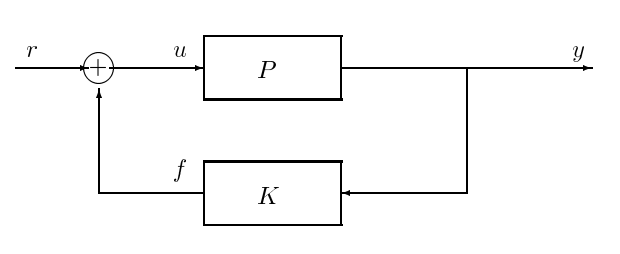
Figure \(PageIndex{1}\): Block diagram of the prototype feedback control configuration.

The plant \(P\) and controller \(K\) could in general be nonlinear, time-varying, and infinite- dimensional, but we shall restrict attention almost entirely to interconnections of finite- order LTI components, whether described in state-space form or simply via their input-output transfer functions. Recall that the transfer functions of such finite-order state-space models are proper rationals, and are in fact strictly proper if there is no direct feedthrough from input to output. We shall use the notation of CT systems in the development that follows, although everything applies equally to DT systems.

The plant and controller should evidently have compatible input/output dimensions; if not, then they cannot be tied together in a feedback loop. For example, if \(P (s)\) is the \(p \times m\) transfer function matrix of the (nominal LTI model of the) plant in Figure 17.1, then the transfer function \(K(s)\) of the (LTI) controller should be an \(m \times p\) matrix.

All sorts of other feedback configurations exist; two alternatives can be found in Figures 17.2 and 17.3. For our purposes in this chapter, the differences among these various configurations are not important.

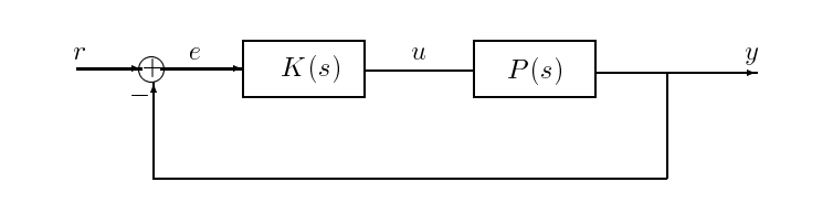
Figure \(PageIndex{2}\): A ("servo") feedback configuration where the tracking error between the command \(r\) and output \(y\) is directly applied to the controller.

Our discussion for now will focus on the arrangement shown in Figure 17.4, which is an elaboration of Figure 17.1 that represents some additional signals of interest. Interpretations for the various (vector) signals depicted in the preceding figures are normally as follows:

• \(u\) - control inputs to plant - control inputs to plant

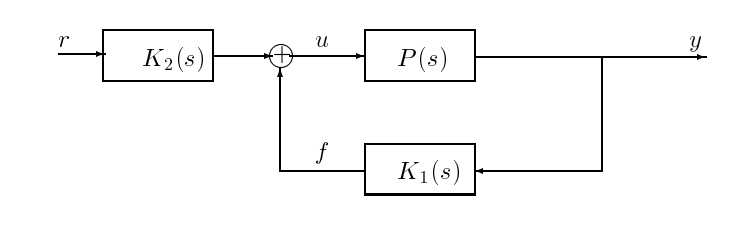
Figure \(PageIndex{3}\): A two-parameter-compensator feedback scheme.

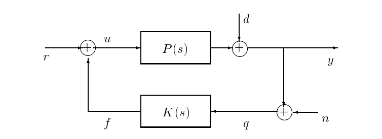
Figure \(PageIndex{4}\): Including plant disturbances \(d\) and measurement noise \(n\).

• \(y\) - measured outputs of plants
• \(d\) - plant disturbances, represented as acting at the output
• \(n\) - noise in the output measurements used by the feedback controller
• \(r\) - reference or command inputs
• \(e\) - tracking error \(r-y\)
• \(f\) - output of feedback compensator

Transfer Functions

We now show how to obtain the transfer functions of the mappings relating the various signals found in Figure 17.4; the transform argument, \(s\), is omitted for notational simplicity. We also depart temporarily from our convention of denoting transforms by capitals, and mark the transforms of all signals by lower case, saving upper case for transfer function matrices (i.e. transforms of impulse responses); this distinction will help the eye make its way through the expressions below, and should cause no confusion if it is kept in mind that all quantities below are transforms. To begin by relating the plant output to the various input signals, we can write

\[\begin{aligned}
y &=P u+d \\
&=P[r+K(y+n)]+d \\
(I-P K) y &=P r+P K n+d \\
y &=(I-P K)^{-1} P r+(I-P K)^{-1} P K n+(I-P K)^{-1} d
\end{aligned}\nonumber\]

Similarly, the control input to the plant can be written as

\[\begin{aligned}
u &=r+K(y+n) \\
&=r+K(P u+d+n) \\
(I-K P) u &=r+K n+K d \\
u &=(I-K P)^{-1} r+(I-K P)^{-1} K n+(I-K P)^{-1} K d
\end{aligned}\nonumber\]

The map \(u \longrightarrow f\) (with the feedback loop open and \(r = 0, n = 0, d = 0\) is given by \(L = KP\), and is called the loop transfer function.

The map \(d \longrightarrow y\) (with \(n = 0, r = 0\)) is given by \(S_{o}=(I-P K)^{-1}\) and is called the output sensitivity function.

The map \(n \longrightarrow y\) (with \(n = 0, r = 0\)) is given by \(T=(I-P K)^{-1}P K\) and is called the complementary sensitivity function.

The map \(r \longrightarrow u\) (with \(d = 0, n = 0\)) is given by \(S_{i}=(I-K P)^{-1}\) and is called the input sensitivity function.

The map \(r \longrightarrow y\) (\(d = 0, n = 0\)) is given by \((I-P K)^{-1} P\) is called the system response function.

The map \(d \longrightarrow u\) (with \(n = 0, r = 0\)) is given by \((I-K P)^{-1} K\)

Note that the transfer function \((I-K P)^{-1} K\) can also be written as \(K(I-P K)^{-1}\), as may be proved by rearranging the following identity:

\[(I-K P) K=K(I-P K)\nonumber\]

Similarly the transfer function \((I-P K)^{-1} P\) can be written as \(P (I-K P)^{-1}\).

Note also that the output sensitivity and input sensitivity functions are different, because, except for the case when \(P\) and \(K\) are both single-input, single-output (SISO), we have

\[(I-K P)^{-1} \neq(I-P K)^{-1}\nonumber\]