19.1: Additive Representation of Uncertainity

It is commonly the case that the nominal plant model is quite accurate for low frequencies but deteriorates in the high-frequency range, because of parasitics, nonlinearities and/or time-varying effects that become significant at higher frequencies. These high-frequency effects may have been left unmodeled because the effort required for system identification was not justified by the level of performance that was being sought, or they may be well-understood effects that were omitted from the nominal model because they were awkward and unwieldy to carry along during control design. This problem, namely the deterioration of nominal models at higher frequencies, is mitigated to some extent by the fact that almost all physical systems have strictly proper transfer functions, so that the system gain begins to roll off at high frequency.

In the above situation, with a nominal plant model given by the proper transfer function P0(s), the actual plant represented by \(P (s)\), and the difference \(P (s) - P_{0}(s)\) assumed to be stable, we may be able to characterize the model uncertainty via a bound of the form

\[\left|P(j \omega)-P_{0}(j \omega)\right| \leq \ell_{a}(\omega) \ \tag{19.1}\]

where

\[\ell_{a}(\omega)=\left\{\begin{aligned}
\text { "Small" } & ;|\omega|<\omega_{c} \\
\text { "Bounded" } & ; \quad|\omega|>\omega_{c}
\end{aligned}\right. \ \tag{19.2}\]

This says that the response of the actual plant lies in a "band" of uncertainty around that of the nominal plant. Notice that no phase information about the modeling error is incorporated into this description. For this reason, it may lead to conservative results.

The preceding description suggests the following simple additive characterization of the uncertainty set:

\[\Omega_{a}=\left\{P(s) \mid P(s)=P_{0}(s)+W(s) \Delta(s)\right\} \ \tag{19.3}\]

where \(\Delta\) is an arbitrary stable transfer function satisfying the norm condition

\[\|\Delta\|_{\infty}=\sup _{\omega}|\Delta(j \omega)| \leq 1 \ \tag{19.4}\]

and the stable proper rational weighting term \(W(s)\) is used to represent any information we have on how the accuracy of the nominal plant model varies as a function of frequency. Figure 19.1 shows the additive representation of uncertainty in the context of a standard servo loop, with \(K\) denoting the compensator.

When the modeling uncertainty increases with frequency, it makes sense to use a weighting function \(W(j \omega)\) that looks like a high-pass filter: small magnitude at low frequencies, increasing but bounded at higher frequencies.

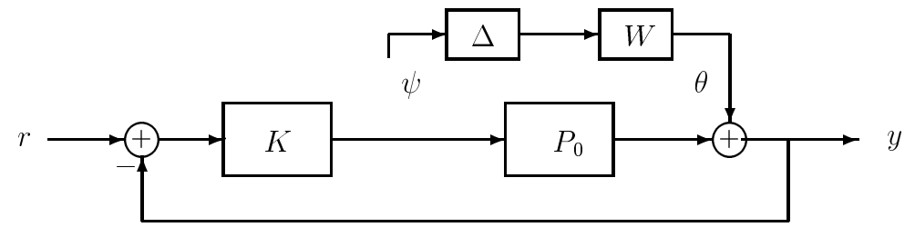
Figure 19.1: Representation of the actual plant in a servo loop via an additive perturbation of the nominal plant.

Caution: The above formulation of an additive model perturbation should not be interpreted as saying that the actual or perturbed plant is the parallel combination of the nominal system \(P_{0}(s)\) and a system with transfer function \(W(s) \Delta(s)\). Rather, the actual plant should be considered as being a minimal realization of the transfer function \(P (s)\), which happens to be written in the additive form \(P_{0}(s)+W(s) \Delta(s)\).

Some features of the above uncertainty set are worth noting:

• The unstable poles of all plants in the set are precisely those of the nominal model. Thus, our modeling and identification efforts are assumed to be careful enough to accurately capture the unstable poles of the system.
• The set includes models of arbitrarily large order. Thus, if the uncertainties of major concern to us were parametric uncertainties, i.e. uncertainties in the values of the parameters of a particular (e.g. state-space) model, then the above uncertainty set would greatly overestimate the set of plants of interest to us

The control design methods that we shall develop will produce controllers that are guaranteed to work for every member of the plant uncertainty set. Stated slightly differently, our methods will treat the system as though every model in the uncertainty set is a possible representation of the plant. To the extent that not all members of the set are possible plant models, our methods will be conservative.

Suppose we have a set of possible plants \(\Pi\) such that the true plant is a member of that set. We can try to embed this set in an additive perturbation structure. First let \(P_{0} \in \Pi\) be a certain nominal plant in \(\Pi\). For any other plant \(P \in \Pi\) we write,

\[P(j \omega)=P_{0}(j \omega)+W(j \omega) \Delta(j \omega)\nonumber\]

The weight \(|W(j \omega)|\) satisfies

\[\begin{aligned}
|W(j \omega)| & \geq|W(j \omega) \Delta(j \omega)|=\left|P(j \omega)-P_{0}(j \omega)\right| \\
|W(j \omega)| & \geq \max _{P \in \Pi}\left|P(j \omega)-P_{0}(j \omega)\right|=\ell_{a}(j \omega)
\end{aligned}\nonumber\]

With the knowledge of the lower bound \(l_{a}(j \omega)\), we find a stable system \(W(s)\) such that \(|W(j \omega)| \geq \ell_{a}(j \omega)\)