19.2: Multiplicative Representation of Uncertainty

Another simple means of representing uncertainty that has some nice analytical properties is the multiplicative perturbation, which can be written in the form

\[\Omega_{m}=\left\{P \mid P=P_{0}(1+W \Delta),\|\Delta\|_{\infty} \leq 1\right\}\ \tag{19.5}\]

\(W\) and \(\Delta\) are stable. As with the additive representation, models of arbitrarily large order are included in the above sets.

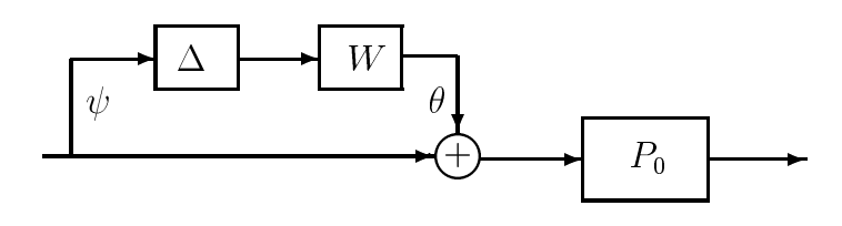
Figure 19.2: Representation of uncertainty as multiplicative perturbation at the plant input

The caution mentioned in connection with the additive perturbation bears repeating here: the above multiplicative characterizations should not be interpreted as saying that the actual plant is the cascade combination of the nominal system P0 and a system \(1 + W \Delta\). Rather, the actual plant should be considered as being a minimal realization of the transfer function \(P (s)\), which happens to be written in the multiplicative form.

Any unstable poles of \(P\) are poles of the nominal plant, but not necessarily the other way, because unstable poles of \(P_{0}\) may be cancelled by zeros of \(I + W \Delta\). In other words, the actual plant is allowed to have fewer unstable poles than the nominal plant, but all its unstable poles are confined to the same locations as in the nominal model. In view of the caution in the previous paragraph, such cancellations do not correspond to unstable hidden modes, and are therefore not of concern.

As in the case of additive perturbations, suppose we have a set of possible plants \(\Pi\) such that the true plant is a member of that set. We can try to embed this set in a multiplicative perturbation structure. First let \(P_{0} \in \Pi\) a certain nominal plant in \(\Pi\). For any other plant \(P \in \Pi\) we have

\[P(j \omega)=P_{0}(j \omega)(1+W(j \omega) \Delta(j \omega))\nonumber\]

The weight \(|W(j \omega)|\) satisfies

\[\begin{aligned}
|W(j \omega)| & \geq|W(j \omega) \Delta(j \omega)|=\left|\frac{P(j \omega)-P_{0}(j \omega)}{P_{0}(j \omega)}\right| \\
|W(j \omega)| & \geq \max _{P \in \Pi}\left|\frac{P(j \omega)-P_{0}(j \omega)}{P_{0}(j \omega)}\right|=\ell_{m}(j \omega)
\end{aligned}\nonumber\]

With the knowledge of the envelope \(l_{m}(j \omega)\), we find a stable system \(W(s)\) such that \(|W(j \omega)| \geq l_{m} (j \omega)\)

Example 19.1 Uncertain gain

Suppose we have a plant \(P=k \bar{P}(s)\) with an uncertain gain \(k\) that lies in the interval \(k_{1} \leq k \leq k_{2}\). We can write \(k=\alpha(1+\beta x)\) such that

\[\begin{array}{l}
k_{1}=\alpha(1-\beta) \\
k_{2}=\alpha(1+\beta)
\end{array}\nonumber\]

Therefore \(\alpha=\frac{k_{1}+k_{2}}{2}\), \(\beta=\frac{k_{2}-k_{1}}{k_{2}+k_{1}}\), and we can express the set of plants as

\[\Pi=\left\{P(s) \mid P(s)=\frac{k_{1}+k_{2}}{2} \bar{P}(s)\left(1+\frac{k_{2}-k_{1}}{k_{2}+k_{1}} x\right),-1 \leq x \leq 1\right\}\nonumber\]

We can embed this \(\Pi\) in a multiplicative structure by enlarging the uncertain elements \(x\) which are real numbers to complex \(\Delta(j \omega)\) representing dynamic perturbations. This results in the following set

\[\Omega_{m}=\left\{P(s) \mid P(s)=\frac{k_{1}+k_{2}}{2} \bar{P}(s)\left(1+\frac{k_{2}-k_{1}}{k_{2}+k_{1}} \Delta\right),\|\Delta\|_{\infty} \leq 1\right\}\nonumber\]

Note that in this representation \(P_{0}=\frac{k_{1}+k_{2}}{2} \bar{P}\), and \(W=\frac{k_{2}-k_{1}}{k_{2}+k_{1}}\)

Example 19.2 Uncertain Delay

Suppose we have a plant \(P=e^{-k s} P_{0}(s)\) with an uncertain delay \(0 \leq k \leq k_{1}\). We want to represent this family of plants in a multiplicative perturbation structure. The weight \(W(s)\) should satisfy

\[\begin{aligned}
|W(j \omega)| & \geq \max _{0 \leq k \leq k_{1}}\left|\frac{e^{-j \omega k} P_{0}(j \omega)-P_{0}(j \omega)}{P_{0}(j \omega)}\right| \\
&=\max _{0 \leq k \leq k_{1}}\left|e^{-j \omega k}-1\right| \\
&=\left\{\begin{array}{cc}
\mid 1-e^{-j \omega k_{1} \mid} & \omega<\frac{\pi}{k_{1}} \\
0 & \omega \geq \frac{\pi}{k_{1}}
\end{array}\right.\\
&=\ell_{m}(\omega)
\end{aligned}\nonumber\]

A stable weight that satisfies the above relation can be taken as

\[W(s)=\alpha \frac{2 \pi k_{1} s}{\pi k_{1} s+1}\nonumber\]

where \(\alpha > 1\). The reader should verify that this weight will work by ploting \(|W(j \omega)|\) and \(l_{m}( \omega)\), and showing that \(l_{m}( \omega)\) is below the curve \(|W(j \omega)|\) for all \(\omega\).