20.3: Multiplicative Representation of Uncertainty

Another simple means of representing uncertainty that has some nice analytical properties is the multiplicative perturbation, which can be written in the form

\[\Omega=\left\{P \mid P=P_{0}(I+W \Delta),\|\Delta\|_{\infty} \leq 1\right\} \ \tag{20.5}\]

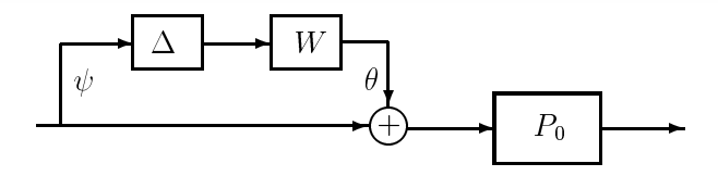
Figure 20.2: Representation of uncertainty as multiplicative perturbation at the plant input.

An alternative to this input-side representation of the uncertainty is the following output-side representation:

\[\Omega=\left\{P \mid P=(I+W \Delta) P_{0},\|\Delta\|_{\infty} \leq 1\right\}\nonumber\]

In both the multiplicative cases above, \(W\) and \(\Delta\) are stable. As with the additive representation, models of arbitrarily large order are included in the above sets. Still other variations may be imagined; in the case of matrix weights, for instance, the term \(W \Delta\) can be replaced by \(W_{1} \Delta W_{2}\).

The caution mentioned in connection with the additive perturbation bears repeating here: the above multiplicative characterizations should not be interpreted as saying that the actual plant is the cascade combination of the nominal system \(P_{0}\) and a system \(I + W \Delta\). Rather, the actual plant should be considered as being a minimal realization of the transfer function \(P (s)\), which happens to be written in the multiplicative form.

Any unstable poles of \(P\) are poles of the nominal plant, but not necessarily the other way, because unstable poles of \(P_{0}\) may be cancelled by zeros of \(I + W \Delta\). In other words, the actual plant is allowed to have fewer unstable poles than the nominal plant, but all its unstable poles are confined to the same locations as in the nominal model. In view of the caution in the previous paragraph, such cancellations do not correspond to unstable hidden modes, and are therefore not of concern.