20.5: A Linear Fractional Description

We start with a given a nominal plant model \(P_{0}\), and a feedback controller \(K\) that stabilizes \(P_{0}\). The robust stability question is then: under what conditions will the controller stabilize all \(P \in \Omega\)? More generally, we assume we have an interconnected system that is nominally internally stable, by which we mean that the transfer function from an input added in at any subsystem input to the output observed at any subsystem output is always stable in the nominal system. The robust stability question is then: under what conditions will the interconnected system remain internally stable for all possible perturbed models.

If the plant uncertainty is specified (additively, multiplicatively, or using a feedback representation) via an uncertainty block of the form \(W \Delta\), where \(W\) and \(\Delta\) are stable, then the actual (closed-loop) system can be mapped into the very simple feedback configuration

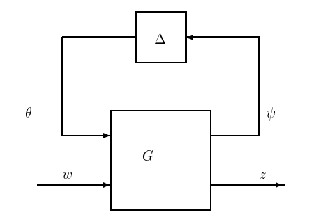
Figure 20.3: Standard model for uncertainty.

shown in Figure 20.3. (The generalization to an uncertainty block of the form \(W_{1} \Delta W_{2}\) is trivial, and omitted here to avoid additional notation.)

As in the previous subsection, the signals \(\psi\) and \(\theta\) respectively denote the input and output of the uncertainty block. The input \(w\) is added in at some arbitrary accessible point of the interconnected system, and \(z\) denotes an output taken from an arbitrary accessible point. An accessible point in our terminology is simply some subsystem input or output in the actual or perturbed system; the input \(\psi\) and output \(\theta\) of the uncertainty block would not qualify as accessible points.

If we remove the perturbation block \(\Delta\) in Fig. 20.3, we are left with the nominal closed-loop system, which is stable by hypothesis (since the compensator \(K\) has been chosen to stabilize the nominal plant and is lumped in \(G\)). Stability of the nominal system implies that the transfer functions relating the outputs \(\psi\) and \(z\) of the nominal system to the inputs \(\theta\) and \(w\) are all stable. Thus, in the transfer function representation

\[\left(\begin{array}{l}
\Psi(s) \\
Z(s)
\end{array}\right)=\left(\begin{array}{cc}
M(s) & N(s) \\
J(s) & L(s)
\end{array}\right)\left(\begin{array}{c}
\Theta(s) \\
W(s)
\end{array}\right) \ \tag{20.7}\]

each of the transfer matrices \(M\), \(N\), \(J\), and \(L\) is stable

Now incorporating the constraint imposed by the perturbation, namely

\[\Theta=(\Delta) \Psi \ \tag{20.8}\]

and solving for the transfer function relating \(z\) to \(w\) in the perturbed system, we obtain

\[G_{w z}(s)=L+J \Delta(I-M \Delta)^{-1} N \ \tag{20.9}\]

Note that \(M\) is the transfer function "seen" by the perturbation \(\Delta\), from the input \(\theta\) that it imposes on the rest of the system, to the output \(\psi\) that it measures from the rest of the system. Recalling that \(w\) and \(z\) denoted arbitrary inputs and outputs at the accessible points of the actual closed-loop system, we see that internal stability of the actual (i.e. perturbed) closed-loop system requires the above transfer function be stable for all allowed \(\Delta\).