1.1: Model Variables and Element Types

Flow and Across Variables 

Modeling of a physical system involves two kinds of variables: flow variables that ‘flow’ through the components, and across variables that are measured across those components.

For example, in electric circuits, potential (voltage) is measured across elements, whereas electrical charge (current) flows through the circuit elements.

In mechanical linkage systems, displacement and velocity are measured across elements, whereas force or effort ‘flows’ through the linkages.

In thermal and fluid systems, heat and mass serve as the flow variables, whereas temperature and pressure constitute the across variables.

A physical element is characterized by the relationship between flow and across variables. The three basic types are the resistive, inductive, and capacitive elements. The terminology, taken from electrical circuits, extends to other types of physical systems as well.

While the resistive element dissipates energy, both the capacitive and inductive elements store energy. For example, a capacitor stores electrical energy and a moving mass stores kinetic energy. The energy storage accords memory to the element that accounts for it dynamic behavior modeled by an ODE.

Let \(q(t)\) denote a flow variable and \(x(t)\) denote an across variable associated with an element; then, the element type is defined by their mutual relationships, described as follows:

Definition: Resistive Element

A resistive element is described by a proportional relationship:

\[x(t)=k\; q(t) \nonumber \]

Figure \(\PageIndex{1}\): A resistive element.

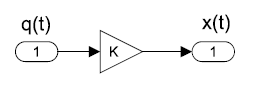
For example, the voltage and current relationship through a resister is described by a proportional relationship called Ohm’s law: \(V(t)=R\; i(t)\).

Similarly, the force–velocity relationship though a linear mechanical damper is a proportional one: \(v(t)=\frac{1}{b} f(t)\).

Definition: Capacitive Element

A capacitive element is described by the relation:

\[x(t)=k\int q(t) dt+x_{0} \nonumber \]

i.e., the across variable varies in proportion to the accumulated amount of the flow variable. Whereas, the flow variable varies proportionally with the rate of change of the across variable:

\[q\left(t\right)=\frac{1}{k}\frac{dx\left(t\right)}{dt} \nonumber \]

Figure \(\PageIndex{2}\): A capacitive element.

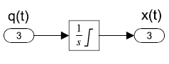
For example, the voltage and current relationship through a capacitor is given as: \(V(t)=\frac{1}{C} \int i(t) dt+V_{0}\). Since the current integral represents the accumulation of electrical charge, we have: \(Q=CV\). The inverse relationship is described as: \(i\left(t\right)=C\frac{dV}{dt}\).

Similarly, the force–velocity relationship that governs the movement of an inertial mass is described as: \(v(t)=\frac{1}{m} \int f(t) dt+v_{0}\). Its inverse is the familiar Newton’s second law of motion: \(f\left(t\right)=m\frac{dv\left(t\right)}{dt}\).

Definition: Inductive Element

An inductive element is described by the relationship:

\[x(t)=k\frac{dq(t)}{dt} \nonumber \]

i.e., the across variable is obtained by differentiating the flow variable. Alternatively, the flow variable varies in proportion to the accumulation of the across variable as:

\[q(t)=\frac{1}{k}\int x(t) dt+q_{0} \nonumber \]

Figure \(\PageIndex{3}\): An inductive element.

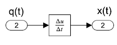
For example, the voltage–current relationship through an inductive coil in an electric circuit is given as: \(V(t)=L\frac{di(t)}{dt}\). The inverse relationship is described as: \(i(t)=\frac{1}{L} \int V(t) dt+i_{0}\).

Similarly, the force–velocity relationship though a linear spring is given as: \(v(t)=\frac{1}{K} \frac{df(t)}{dt}\). The inverse relation is described as: \(f\left(t\right)=K\int{v\left(t\right)dt}+f_0\).