1.5: Industrial Process Models

Last updated
Save as PDF

Page ID: 24389

\( \newcommand{\vecs}[1]{\overset { \scriptstyle \rightharpoonup} {\mathbf{#1}} } \) \( \newcommand{\vecd}[1]{\overset{-\!-\!\rightharpoonup}{\vphantom{a}\smash {#1}}} \)\(\newcommand{\id}{\mathrm{id}}\) \( \newcommand{\Span}{\mathrm{span}}\) \( \newcommand{\kernel}{\mathrm{null}\,}\) \( \newcommand{\range}{\mathrm{range}\,}\) \( \newcommand{\RealPart}{\mathrm{Re}}\) \( \newcommand{\ImaginaryPart}{\mathrm{Im}}\) \( \newcommand{\Argument}{\mathrm{Arg}}\) \( \newcommand{\norm}[1]{\| #1 \|}\) \( \newcommand{\inner}[2]{\langle #1, #2 \rangle}\) \( \newcommand{\Span}{\mathrm{span}}\) \(\newcommand{\id}{\mathrm{id}}\) \( \newcommand{\Span}{\mathrm{span}}\) \( \newcommand{\kernel}{\mathrm{null}\,}\) \( \newcommand{\range}{\mathrm{range}\,}\) \( \newcommand{\RealPart}{\mathrm{Re}}\) \( \newcommand{\ImaginaryPart}{\mathrm{Im}}\) \( \newcommand{\Argument}{\mathrm{Arg}}\) \( \newcommand{\norm}[1]{\| #1 \|}\) \( \newcommand{\inner}[2]{\langle #1, #2 \rangle}\) \( \newcommand{\Span}{\mathrm{span}}\)\(\newcommand{\AA}{\unicode[.8,0]{x212B}}\)

Industrial Process Models

Industrial processes comprise exchange of chemical, electrical or mechanical energy in the manufacturing of industrial products. An industrial process model in its simplified form is represented by a first-order lag with a dead-time that represents the time delay between the application of input and the appearance of the process output.

Let \(\tau\) represent the time constant associated with an industrial process, \(\tau _ d\) represent the dead-time, and \(K\) represent the process dc gain; then, simplified industrial process dynamics are represented by the following delay-differential equation:

\[\tau \frac{ dy(t)}{ dt} +y(t)=Ku(t-t_{d} ) \nonumber \]

Application of the Laplace transform produces the following first-order-plus-dead-time (FOPDT) model of an industrial process:

\[G(s)=\frac{Ke^{-\tau _ d s} }{\tau s+1} \nonumber \]

where the process parameters \(\{ K,\; \tau ,\; \tau _ d \}\), can be identified from the process response to inputs. An rational process model is obtained by using a Taylor series approximation of the delay term, \(e^{-\tau _ d s}\). Typical such approximations include:

\[ e^{-\tau_d s} \simeq 1-\tau _ d s, \ \ \ e^{-\tau _ d s} = \frac{1}{e^{\tau _d s} } \simeq \frac{1}{1+\tau _d s}, \ \ \ e^{-\tau _ds}=\frac{e^{-\tau _ds/2}}{e^{\tau _ds/2}}\simeq \frac{1-\tau _ds/2}{1+\tau_ds/2} \nonumber \]

The last expression is termed as first-order Pade’ approximation and is often preferred. Higher order approximations can also be used.

Example \(\PageIndex{1}\)

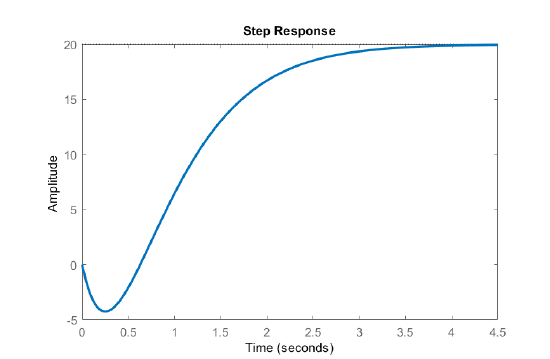
The process parameters of a stirred-tank bioreactor are given as: \(\{ K,\; \tau ,\; \tau _ d \} =\left\{20,0.5,1\right\}\). The transfer function model of the process is formed as:

\[G(s)=\frac{20e^{-s} }{0.5s+1}.\]

By using a first-order Pade’ approximation, a rational transfer function model of the industrial process with delay is obtained as:

\[G(s)=\frac{20\left(1-0.5s\right)}{\left(0.5s+1\right)^{2} }.\]

The step response of the bioreactor transfer function with Pade’ approximation shows an undershoot due to the presence of right half-plane (RHP) zero in the transfer function.

Figure \(\PageIndex{1}\): Step response of the bioreactor model with Pade’ approximation.

pkg load control
s=tf('s');
Gs=20*(1-.5*s)/(1+.5*s)^2;
step(Gs)