2.2: System Natural Response

 

System Natural Response

The transfer function of a dynamic linear time-invariant (LTI) system is given as a ratio of polynomials: \(G(s)=\frac{n(s)}{d(s)}\). The poles of the transfer function are the roots of the denominator polynomial \(d(s)\).

The poles of the transfer function characterize the natural response modes of the system. Thus, if \(p_i\) is a pole of the transfer function, \(G\left(s\right)\), then \(\left\{e^{p_it}\right\}\) constitutes a natural response mode.

• A real pole: \(p_i=-\sigma\), contributes a term \(e^{-\sigma t}\) to system natural response.
• A pair of complex poles: \(p_i=-\sigma \pm j\omega\), contributes oscillatory terms of the form \(e^{-\sigma t}e^{j\omega t}=e^{-\sigma t}\left( \cos \omega t +j \sin \omega t\right)\) to the natural response.

The natural response of the system is a weighted sum of the natural response modes, i.e., \(y_n(t)=\sum_{i=1}^n C_i e^{p_it}\). Further, the natural response is reflected in the impulse response of a system.

Definition: Impulse Response

The impulse response of a system, represented by \(G(s)\), is defined as system response to a unit-impulse input, \(\delta \left(t\right)\), when the initial conditions are zero.

Let \(u\left(t\right)=\delta \left(t\right),\ \ u\left(s\right)=1\); then, the impulse response is computed as: \(y\left(s\right)=G(s)\); in the time-domain, the impulse response is given as: \(g(t)={\rm L}^{-1} \left[G(s)\right]\).

To proceed further, let the system transfer function be represented in the factored form as:

\[G\left(s\right)=\frac{n(s)}{\prod^n_{i=1}{\left(s-p_i\right)}} \nonumber \]

where \(n(s)\) is the numerator polynomial, and \(p_i,\ i=1,\dots n\), are the system poles, assumed to be distinct and may include a single pole at the origin. Using partial fraction expansion (PFE), the impulse response is given as:

\[y_{imp}\left(s\right)=\sum^n_i{\frac{A_i}{s-p_i}} \nonumber \]

Using the inverse Laplace transform, the impulse response of the system is computed as:

\[y_{imp}\left(t\right)=\left(\sum^n_i{A_ie^{p_it}}\right)u(t) \nonumber \]

where \(u(t)\) represents the unit-step function, used here to indicate that the expression for \(g(t)\) is valid for \(t\ge 0\).

Impulse Response of Low Order Systems

First-Order System 

Let \(G(s)=\frac{1}{\tau s+1}\); the system has a signle response mode given as: \(\{e^{-t/\tau }\}\). Thus, the impulse response of the first-order system is computed as: \[g(t)=\frac{1}{\tau }e^{-t/\tau } u(t) \nonumber \]

Example \(\PageIndex{1}\)

The impulse response of \(G(s)=\frac{1}{s+1}\) is given as: \(g(t)=e^{-t}u(t)\).

The impulse response begins at \(g(0)=1\) and asymptotically approaches \(g(\infty)=0\).

pkg load control
s=tf('s');
Gs=1/(s+1);
impulse(Gs), grid on

Definition: System Time Constant

The time constant, \(\tau\), describes the time when, starting from unity, the natural response decays to \(e^{-1}\cong 0.37\), or 37% of its initial value. For a first-order system, with a real pole, \(s=-\sigma\), the time constant is given as: \(\tau =\frac{1}{\sigma }\).

Second-Order System with an Integrator 

Let: \(G(s)=\frac{1}{s\left(\tau s+1\right)}\); then, the natural response modes are: \(\left\{1,\ e^{-t/\tau }\right\}\). The transfer function is expanded using PFE as: \(G(s)=\frac{1}{s} +\frac{\tau }{\tau s+1}\). The impulse response is expressed as: \[g(t)=\left(1-e^{-t/\tau } \right)\, u(t) \nonumber \]

Example \(\PageIndex{2}\)

The impulse response of \(G(s)=\frac{1}{s(s+1)}=\frac{1}{s}-\frac{1}{s+1}\) is given as: \(g(t)=(1-e^{-t}) u(t)\).

The impulse response begins at \(g(0)=0\) and asymptotically approaches \(g(\infty)=1\).

pkg load control
s=tf('s');
Gs=1/s/(s+1);
impulse(Gs), grid on

Second-Order System with Real Poles 

Let \(G\left(s\right)=\frac{1}{\left(s+\sigma_1\right)\left(s+\sigma_2\right)}\); then, the system natural response modes are: \(\left\{e^{-\sigma_1t},\ e^{-\sigma_2t}\right\}\). Assuming \(\sigma_2 \ge \sigma_1\), and using PFE followed by inverse Laplace transform, the system impulse response is expressed as: \[g(t)=\frac{1}{\sigma_2-\sigma_1}\left(e^{-\sigma_1t} -e^{-\sigma_2t} \right)\, u(t) \nonumber \]

Example \(\PageIndex{3}\)

The impulse response of \(G(s)=\frac{1}{(s+1)(s+2)}\) is given as: \(g(t)=(e^{-t}-e^{-2t}) u(t)\).

The impulse response begins at \(g(0)=0\) and asymptotically approaches \(g(\infty)=0\).

pkg load control
s=tf('s');
Gs=1/(s+1)/(s+2);
impulse(Gs), grid on

Second-Order System with Complex Poles 

Let \(G\left(s\right)=\frac{1}{{\left(s+\sigma \right)}^2+{\omega}^2}\); then, by using Euler’s identity, its natural response modes are given as: \(\left\{e^{-\sigma t}{\cos \omega t\ },\ \ e^{-\sigma t}{\sin \omega t\ }\right\}\). Its impulse response is given as: \[g(t)=\frac{1}{\omega } e^{-\sigma t} \; \sin (\omega t)\, u(t) \nonumber \]

The oscillatory natural response is contained in the envelope defined by: \(\pm e^{-\sigma t}\). The effective time constant of a second-order system is given as: \({\tau }_{eff}=\frac{1}{\sigma }\).

The natural response is of the form: \(y_n\left(t\right)=(C_1{\cos \omega t\ }+C_2{\sin \omega t\ })e^{-\sigma t}\) can be alternatively expressed as: \[y_n\left(t\right)=Ce^{-\sigma t}{sin \left(\omega t+\phi \right)\ } \nonumber \] where \(C=\sqrt{C^2_1+C^2_2}\) and \({tan \phi \ }=\frac{C_1}{C_2}\).

Example \(\PageIndex{4}\)

The impulse response of \(G(s)=\frac{s}{s^2+2s+2}=\frac{s}{(s+1)^2+1^2}=\frac{s+1-1}{(s+1)^2+1^2}\) is given as: \[g(t)=(\cos t-\sin t)e^{-t} u(t)=\sqrt{2}\sin (t+135^{\circ}) u(t)=\sqrt{2}\cos (t+45^{\circ})u(t) \nonumber \]

The impulse response begins at \(g(0)=\cos(0)=1\) and asymptotically approaches \(g(\infty)=0\).

pkg load control
s=tf('s');
Gs=s/(s^2+2*s+2);
impulse(Gs), grid on

 

Figure \(\PageIndex{1}\): Impulse response of transfer function models: (a) first-order system; (b) second-order system with a pole at the origin; (c) second-order system with real poles; and, (d) second-order system with complex poles.

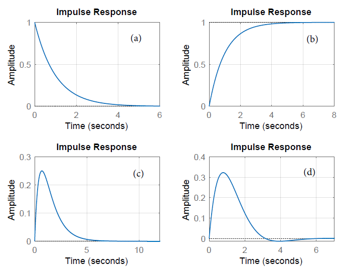
From the figure, we may observe that:

1. While the impulse response of a first-order system starts from a value of unity, the impulse response of a second-order system starts from zero.
2. The impulse response of a stable system with poles in the open left-half plane (OLHP), \(Re\left(p_i\right)<0\), asymptotically dies out with time, i.e., \({\mathop{lim}_{t\to \infty } g\left(t\right)=0\ }\).
3. ; the impulse response of a system with a pole at the origin approaches a constant value of unity in the steady-state (which represents the integral of the delta function). Such systems are termed marginally stable.