2.5: Sinusoidal Response of a System
- Page ID
- 24397

Response to Sinusoidal Input
The sinusoidal response of a system refers to its response to a sinusoidal input: \(u(t)=\cos \; \omega _{0} t\) or \(u(t)=\sin \; \omega _{0} t\).
To characterize the sinusoidal response, we may assume a complex exponential input of the form: \(u\left(t\right)=e^{j{\omega }_0t},\ \ u\left(s\right)=\frac{1}{s-j{\omega }_0}\). Then, the system output is given as: \(\ y\left(s\right)=\frac{G\left(s\right)}{s-j{\omega }_0}\).
To proceed, let \(G\left(s\right)=\frac{n(s)}{\prod^n_{i=1}{\left(s-p_i\right)}}\), where \(p_i,\ i=1,\dots n\), denote the poles of the transfer function; then, using PFE, the system response is given as:
\[y\left(s\right)=\frac{A_0}{s-j{\omega }_0}+\sum^n_{i=1}{\frac{A_i}{s-p_i}} \nonumber \]
where \(A_0=G\left(j{\omega }_0\right)\). The time response of the system is given as: \[y\left(t\right)=G\left(j{\omega }_0\right)e^{j{\omega }_0t}+\sum^n_{i=1}{A_ie^{p_it}} \nonumber \]
Assuming BIBO stability, i.e., \(Re\left[p_i\right]<0\), the transient response component dies out with time. Then, the steady-state response is described as: \[y_{ss}(t)=G\left(j{\omega }_0\right)e^{j{\omega }_0t} \nonumber \]
The frequency response function, for a given transfer function \(G(s)\) is defined as: \(G(j\omega )=G(s)|_{s=j\omega }\).
The frequency response function is described in the magnitude-phase form as: \(G(j\omega )=\left|G(j\omega )\right|e^{\angle G(j\omega )} .\)
When computed at a particular frequency, \(\omega ={\omega }_0\), the frequency response function, \(G\left(j{\omega }_0\right)\) is a complex number.
Then, the steady-state response to a complex sinusoid \(u(t)=e^{j\omega _{0} t}\) is given as: \[y_{ss} (t)=\left|G(j\omega _{0} )\right|e^{\angle G(j\omega_0 )} e^{j\omega _{0} t} \nonumber \]
By Euler’s identity, we have: \(e^{j\omega _{0} t} =\cos \left(\omega _{0} t\right)+j\,\;\sin \left(\omega _{0} t\right)\); therefore, the steady-state response to \(u(t)=\cos \, \omega _{0} t\) is given as: \[y_{\rm ss} (t)=\left|G(j\omega _{0} )\right|\cos (\omega _{0} t+\angle G(j\omega _{0} )) \nonumber \]
Similarly, the steady-state response to \(u(t)=\sin \, \omega _{0} t\) is given as: \[y_{\rm ss} (t)=\left|G(j\omega _{0} )\right|\,\sin (\omega _{0} t+\angle G(j\omega _{0} )) \nonumber \]
Thus, the steady-state response to sinusoid of a certain frequency is a sinusoid at the same frequency, scaled by the magnitude of the frequency response function; the response includes a phase contribution from the frequency response function.
Examples
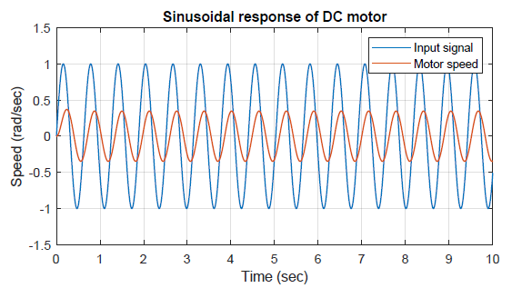
A small DC motor model is approximated as: \(G\left(s\right)=\frac{500}{\left(s+10\right)\left(s+100\right)}\).
Its frequency response function is given as: \(G\left(j\omega \right)=\frac{0.5}{\left(0.01\omega +1\right)\left(0.1\omega +1\right)}\).
Let \(u(t)=\sin 10t\); then, in the steady-state, the sinusoidal response is given as: \(y_{ss}\left(t\right)=0.35\;{\sin \left(10t-50{}^\circ \right)\ }\).
The sinusoidal response of the DC motor is plotted in Figure 2.5.1.
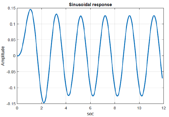
The model of a mass–spring–damper system is given as: \(G\left(s\right)=\frac{1}{s^2+2s+5}=\frac{1}{{\left(s+1\right)}^2+2^2}\); the complex poles are located at: \(s=-1\pm j2\).
Let \(u(t)=\sin \; \pi t\); then, in the steady-state, we have: \(y_{ss}\left(t\right)=0.126\;{\sin \left(\pi t-128{}^\circ \right)\ }\).
The response is plotted below and includes the transient response, which dies out in 4-5 sec.
Visualizing the Frequency Response
The frequency response function is given in polar form as: \(G(j\omega )=|G(j\omega )|e^{j\phi (\omega )}\).
As \(\omega\) varies from \(0\) to \(\infty\), both magnitude and phase may be plotted as functions of \(\omega\).
It is customary to plot both magnitude and phase against \({\log \;\omega \ }\), which accords a high dynamic range to \(\omega\). Further, the magnitude is plotted in decibels as: \(|G(j\omega )|_{\rm dB} =20\; \log _{10} |G(j\omega )|\). The phase \(\phi (\omega )\) is plotted in degrees. The resulting frequency response plots are commonly known as Bode plots.
The plotting of the frequency response in the case of first and second-order systems is illustrated below.
First-Order System
Let \(G(s)=\frac{K}{\tau s+1} \;\); then \(G\left(j\omega \right)=\frac{K}{1+j\omega \tau }\); Hence,
\[{\left|G\left(j\omega \right)\right|}_{\rm dB}=20\;{\log K\ }-20\;{\log \left|1+j\omega \tau \right|\ },\;\;\; \angle G\left(j\omega \right)=-{{\tan}^{-1} \omega \tau \ } \nonumber \]
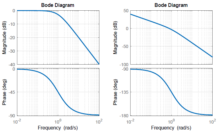
The Bode magnitude and phase plots for \(G\left(s\right)=\frac{1}{s+1}\) are plotted (Figure 2.5.3).
The magnitude plot is characterized by: \(G\left(j0\right)=0 \;{\rm dB},\ \ G\left(j1 \right)=-3 \;{\rm dB}\), and a \(-20 \;{\rm dB}/{\rm decade}\) slope for large \(\omega\).
The phase plot is characterized by: \(G\left(j0\right)=0{}^\circ ,\ G\left(j{0.1}\right)=-5.7{}^\circ ,\ G\left(j1\right)=-45{}^\circ ,\ \ G\left(j10\right)=-84.3{}^\circ ,\ G\left(j\infty \right)=-90{}^\circ\).
First-Order System with Integrator
Let \(G(s)=\frac{K}{s\left(\tau s+1\right)}\); then \(G\left(j\omega \right)=\frac{K}{j\omega \left(1+j\omega \tau \right)}\); Hence,
\[{\left|G\left(j\omega \right)\right|}_{\rm dB}=20\;{\log K\ }-20\;{\log \omega \ }-20\;{\log \left|1+j\omega \tau \right|\ } \nonumber \]
\[\angle G\left(j\omega \right)=-{{\tan}^{-1} \omega \tau \ }-90{}^\circ \nonumber \]
The Bode magnitude and phase plots for \(G\left(s\right)=\frac{1}{s\left(s+1\right)}\) are plotted below.
The magnitude plot is characterized by an initial slope of \(-20 \;{\rm dB}/{\rm decade}\) that changes to \(-40 \;{\rm dB}/{\rm decade}\) for large \(\omega\); at the corner frequency, \(G\left(j1 \right)=-3 \;{\rm dB}\).
The phase plot is characterized by: \(G\left(j0\right)=-90{}^\circ ,\ G\left(j{0.1}\right)=-96{}^\circ ,\ G\left(j1\right)=-135{}^\circ ,\ \ G\left(j10\right)=-174.3{}^\circ ,\ G\left(j\infty \right)=-180{}^\circ\).
Second-Order System with Real Poles
Let \(G(s)=\frac{K}{(\tau _{1} s+1)(\tau _{2} s+1)}\); then \(G\left(j\omega \right)=\frac{K}{\left(1+j\omega {\tau }_1\right)\left(1+j\omega {\tau }_2\right)}\); Hence,
\[{\left|G\left(j\omega \right)\right|}_{\rm dB}=20\;{\log K\ }-20\;{\log \left|1+j\omega {\tau }_1\right|\ }-20\;{\log \left|1+j\omega {\tau }_2\right|\ } \nonumber \]
\[\angle G\left(j\omega \right)=-{{\tan}^{-1} \omega {\tau }_1\ }-{{\tan}^{-1} \omega {\tau }_2\ } \nonumber \]
The Bode magnitude and phase plots for \(G\left(s\right)=\frac{2}{\left(s+1\right)\left(s+2\right)}\) are plotted in Figure 2.5.4.
The magnitude plot is characterized by: \(G\left(j0\right)=0 \;{\rm dB},\ \ G\left(j1\right)=-3 \;{\rm dB}\), an intermediate slope of \(-20 \;{\rm dB}/{\rm decade}\), \(G\left(j2\right)=-14 \;{\rm dB}\), and a slope of \(-40 \;{\rm dB}/{\rm decade}\) for large \(\omega\).
The phase plot is characterized by: \(G\left(j0\right)=0{}^\circ ,\ G\left(j1\right)=-45{}^\circ ,\ \ G\left(j2\right)=-135{}^\circ ,\ \ G\left(j\infty \right)=-180{}^\circ\).
Second-Order System with Complex Poles
Let \(G\left(s\right)=\frac{{\omega }^2_n}{s^2+2\zeta {\omega }_ns+{\omega }^2_n}\); then \(G\left(j\omega \right)=\frac{{\omega }^2_n}{{\omega }^2_n-{\omega }^2+j2\zeta \omega {\omega }_n}\), where \({\omega }_n\) and \(\zeta\) represent the natural frequency and the damping ratio. Hence,
\[{\left|G\left(j\omega \right)\right|}_{\rm dB}=-20\;{{\log}_{10} \left|1-{\left(\frac{\omega }{{\omega }_n}\right)}^2+j2\zeta \left(\frac{\omega }{{\omega }_n}\right)\right|\ } \nonumber \]
\[\phi \left(\omega \right)={{\tan}^{-1} \left(\frac{2\zeta \left(\frac{\omega }{{\omega }_n}\right)}{\left[1-{\left(\frac{\omega }{{\omega }_n}\right)}^2\right]}\right)\ } \nonumber \]
The Bode magnitude and phase plots for \(G(s)=\frac{10}{s^{2} +2s+10}\)are plotted below.
The magnitude plot is characterized by: \(G\left(j0\right)=0 \;{\rm dB},\ \ G\left(j{\omega }_n\right)=-20\;{\log \left(2\zeta \right)\ }\), and a \(-40 \;{\rm dB}/{\rm decade}\) slope for large \(\omega\).
The phase plot is characterized by: \(\phi \left(j0\right)=0{}^\circ ,\ \ \phi \left(j{\omega }_n\right)=-90{}^\circ ,\ \ \phi \left(j\infty \right)=-180{}^\circ\).
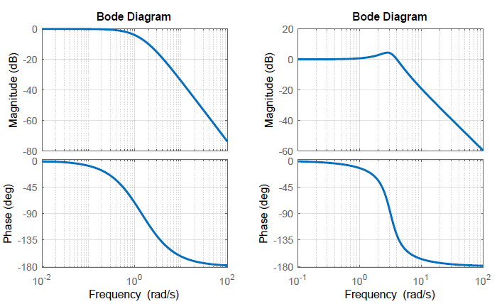
Resonance Peak in the Frequency Response
The Bode magnitude plot of a transfer function with complex poles and low damping displays a distinctive peak in the Bode magnitude plot at the resonant frequency, \({\omega }_r\); the resonant frequency and peak magnitude are computed as:
\[\omega _{r} =\omega _{n} \sqrt{1-2\zeta ^{2} } ,\; \; \zeta <\frac{1}{\sqrt{2} } \nonumber \]
\[M_{\rm p\omega } =\frac{1}{2\zeta \sqrt{1-\zeta ^{2} } } ,\; \; \zeta <\frac{1}{\sqrt{2} } \nonumber \]
Let \(G(s)=\frac{10}{s^{2} +2s+10}\); then, we have: \(\omega _{n} =\sqrt{10} \; \frac{\rm rad}{\rm sec} ,\; \, \zeta =\frac{1}{\sqrt{10} } ,\, \; \omega _{r} =8\; \frac{\rm rad}{\rm sec} ,\;\)and \(M_{\rm p\omega } =1.67\) or \(4.44\; \rm dB\) (Figure 2.5.4).
Relating the Time and Frequency Response
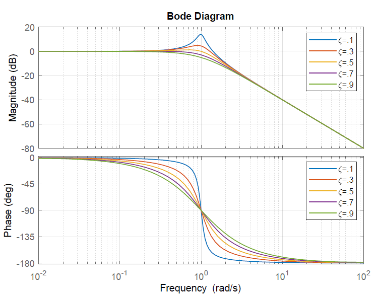
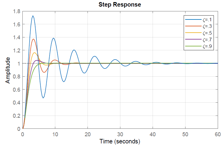
When the system transfer function has poles with a low damping ratio, the Bode magnitude plot displays a resonant peak. Concurrently, the step response of the system displays oscillations.
To illustrate this relationship, we consider a prototype second-order systems: \(G(s)=\frac{1}{s^{2} +2\zeta s+1}\), where \(\omega _{n} =1\), \(\zeta \in \left\{0.1,\, 0.3,\, 0.5,\, 0.7,\, 0.9\right\}\).
The frequency response and the time-domain unit-step response for the second-order transfer functions with \(\omega _{n} =1\) for the various values of \(\zeta \in \left\{0.1,\, 0.3,\, 0.5,\, 0.7,\, 0.9\right\}\) are plotted below.