4.2: Transient Response Improvement

Transient Response Improvement

We consider the feedback control system (Figure 4.2.1) with input \(r(s)\) and output \(y(s)\). 

Figure \(\PageIndex{1}\): Copy and Paste Caption here. (Copyright; author via source)

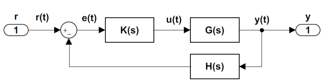
The closed-loop system response is given as: \(y(s)=T(s)r(s)\), where  \(T(s)=\frac{KG(s)}{1+KGH(s)} \).

The system response consists of transient and steady-state components, i.e.,  \(y(t)=y_{tr}(t)+y_{ss}(t)\).

In particular, for a constant input, \(r_{ss}\), the steady-state component of the system response is given as: \(y_{ss}=T(0)r_{ss}\).

The transient response is characterized by the roots of the closed-loop characteristic polynomial, given as: \(\Delta(s)=1+KGH(s)\). 

These roots can be real or complex, distinct or repeated. Accordingly, the system natural response modes are characterized as follows:

Real and Distinct Roots. Let \(\Delta (s)=(s-p_{1} )(s-p_{2} )\ldots (s-p_{n} ).\); then, the system natural response modes are given as: \(\left\{e^{p_{1} t} ,e^{p_{2} t} ,\; \ldots \, ,e^{p_{n} t} \right\}\).

Real and Repeated Roots. Let \(\Delta _{m} (s)=(s-s_{1} )^{m}\); then, the corresponding natural response modes is given as: \(\left\{e^{s_{1} t} ,\; te^{s_{1} t} ,\; \ldots ,\; t^{m-1} e^{s_{1} t} \right\}\).

Complex Roots. Let \(\Delta _ c (s)=(s+\sigma )^{2} +\omega ^{2} \); then, the corresponding natural response modes are given as: \(\left\{e^{-\sigma t} \cos \omega t\; ,\; \; e^{-\sigma t} \sin \omega t\right\}\).

General Expression. Assume that for an \(n\)th order polynomial, the response modes are given as: \(\phi _{k} (t),\; k=1,\ldots ,n\). Then, using arbitrary constants, \(c_{k}\), the system natural response is given as: \(y(t)=\sum _{k=1}^{n} c_{k} \phi _{k} (t)\nonumber\).

Control System Design Specifications

The control system design specifications include desired characteristics for the transient and steady-state components of system response with respect to a prototype input. A step input is used to define the desired transient response characteristics. 

The qualitative indicators of the step response include the following:

1. The rise time (\(t_{r}\))
2. The peak time (\(t_{p}\))
3. The response peak (\(M_p\)) and percentage overshoot (%OS),
4. The settling time (\(t_{s}\))

Rise Time. For overdamped systems (\(\zeta >1\)), the rise time is the time taken by the response to reach from \(10\%\) to \(90\%\) of its final value. For underdamped systems (\(\zeta <1\)), the rise time is the time when the response first reaches its steady-state value.

Peak Time. For underdamped systems, the peak time is the time when the step response reaches its peak.

Peak Overshoot. The peak overshoot is the overshoot above the steady-state value.

Settling Time. The settling time is the time when the step response reaches and stays within \(2\%\) of its steady-state value. Alternately, \(1\%\) limits can be used.

Prototype Second-Order System

To illustrate the above characteristics, we consider a prototype second-order transfer function, given by the closed-loop transfer function as: \[T\left(s\right)=\frac{{\omega }^2_n}{s^2+2\zeta {\omega }_ns+{\omega }^2_n} \nonumber \]

The poles for the prototype system are located at: \(s=-\zeta {\omega }_n\pm j{\omega }_d\), where \({\omega }_d={\omega }_n\sqrt{1-{\zeta }^2}\) is the damped natural frequency.

The impulse and the step response of the prototype system are given as: \[y_{imp}(t)=\frac{{\omega }^2_n}{{\omega }_d} e^{-\zeta {\omega }_nt}{\sin \left({\omega }_dt\right)\ }u(t) \nonumber \]

\[y_{step}(t)=T(0) \left(1-e^{-\zeta {\omega }_n t} \sin \, (\omega _{d} t+\phi)\right)\, u(t),\, \, \, \phi =\tan ^{-1} \frac{\omega_d }{\zeta\omega _n } \nonumber \]

For the prototype system, the rise time, \(t_r\), is indicated by \({\omega }_dt_r+\phi =\pi\). Thus, \(t_r=\frac{\pi -\phi }{{\omega }_d}\); the rise time is bounded as: \(\frac{\pi }{2{\omega }_d}\le t_r\le \frac{\pi }{{\omega }_d}\).

The peak time is indicated by \({\omega }_dt_p=\pi\); thus, \(t_p=\frac{\pi }{{\omega }_d}\).

The peak overshoot is given as: \(M_p=1+e^{-\zeta {\omega }_nt_p}\); the percentage overshoot is given as: \(\%OS=100e^{-\zeta {\omega }_nt_p}\).

The effective time constant of the prototype system is: \(\tau =\frac{1}{\zeta {\omega }_n}\). The step response reaches and stays within \(2\%\) of its final value in about \(4\tau\), and within \(1\%\) of its final value in about \(4.5\tau\).

These metrics are summarized in the Table below.

Table 2.1: Quality metrics used to measure second-order system response.

Quality indicator	Expression
Rise time	\(t_r=\frac{\pi -\phi }{{\omega }_d},\ \ \phi ={{tan}^{-1} \frac{\sqrt{1-{\zeta }^2}}{\zeta }\ }\)
Peak time	\(t_p=\frac{\pi }{{\omega }_d}\)
Peak overshoot	\(M_p=100e^{-\zeta {\omega }_nt_p}(\%)\)
Settling time	\(t_s\cong \frac{4.5}{\zeta {\omega }_n}\)

We may note that the above step response quality indicators are all functions of the damping ratio, \(\zeta\), of the closed-loop roots.

To clarify this relationship, the variation in the step overshoot, \(\% { OS}\), and the normalized rise time, \({\omega }_nt_r\), with \(\zeta\) is tabulated below for selected values of \(\zeta\).

Table 2.2: Percentage overshoot and rise time vs. damping ratio 

\(\zeta\)	0.9	0.8	0.7	0.6	0.5
\(\% { OS}\)	0.2%	1.5%	4.6%	9.5%	16.3%
\({\omega }_nt_r\)	5.54	4.18	3.3	2.76	2.42

A low (\(\le 10\%\)) overshoot in the step response is often desired, which translates into \(\zeta \ge 0.6.\)

Example \(\PageIndex{1}\)

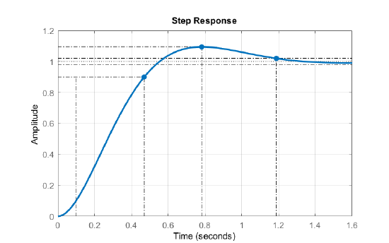
For a prototype second-order system, let \(T\left(s\right)=\frac{25}{s^2+6s+25}\). The closed-loop poles are located at: \(p_{1,2}=-3\pm j4\), hence \({\omega }_n=5\frac{rad}{s}\) and \(\zeta =0.6\).

The step response of the system displays: \(t_r\cong 0.47\,sec, \;t_p\cong 0.78\,sec, \;\%OS=9\%\), and \(t_s\cong 1.19\,sec \) (\(2\%\) threshold).

Figure \(\PageIndex{1}\): Step response of a prototype second-order system showing rise time, peak time and settling time. 

Desired Closed-Loop Characteristic Polynomial

The system design specifications, expressed in terms of rise time (\(t_r\)), settling time (\(t_ s\)), damping ratio (\(\zeta\)), and percentage overshoot (\(\% { O}S\)), are used to define desired root locations for the closed-loop characteristic polynomial.

In particular, assuming a root root location, \(-\sigma \pm j\omega\), the following restrictions are placed on the real and imaginary parts:

1. The settling time constraint places a bound on the real part of the roots: \(\sigma \ge \frac{4.5}{t_s}\).
2. The damping ratio constraint requires that: \(\theta \le \pm \cos ^{-{ 1}} \zeta\), where \(\theta\) is the angle of the desired root location from the origin of the complex plane.
3. The rising time constraint places a bound on the natural frequency of the closed-loop roots as \({\omega }_n\ge \frac{2}{t_r}\).

These constraints are summarized below:

\[\sigma \ge \frac{4.5}{t_s},\ \ {\omega }_n\ge \frac{2}{t_r},\ \ \theta \le\cos^{-1} \zeta \nonumber \]

Example \(\PageIndex{2}\)

We assume the following design specifications: \(0.7<\zeta <1\) and \(t_{s} <2s\). Then, the desired region for the closed-loop root locations is bounded by: \(\sigma \ge 2\) and \(\theta \le \pm 45^{\circ }\).

Figure \(\PageIndex{2}\): The desired region for closed-loop pole placement for \(0.7<\zeta <1\) and \(t_ s <2\)s.

 

Example \(\PageIndex{3}\)

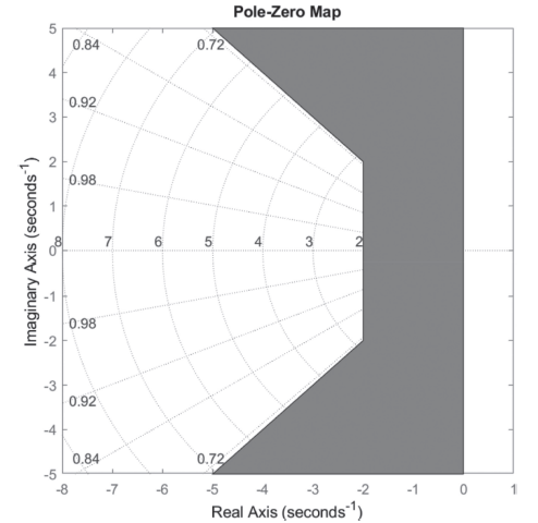
Assume that the design specifications are specified as: \(t_r \le 0.5 s\), \(t_ s \le 3.0 s\), and % \({ \% O}S\le 10\%\). These specifications place the following constraints on the closed-loop pole locations: \(\sigma \ge 1.5,\ {\omega }_n\ge 4,\) and \(\zeta \ge 0.6\).

To meet the constraints, we may choose, e.g., the desired closed-loop characteristic polynomial as: \(\Delta_{des}(s)=(s+\sigma )^2+{\omega }^2_d=s^2+6s+20\).

Controller Gain Selection

The closed-loop characteristic polynomial for a unity-gain feedback system includes static controller gain, \(K\), as a parameter. The characteristic polynomial is given as: \(\Delta(s,K)=1+KG(s)\).

Given a desired characteristic polynomial, \(\Delta_{des}(s)\), we may choose the controller gain by comparing the coefficients of the two polynomials.

Example \(\PageIndex{4}\)

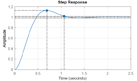
The simplified model of a small DC motor is given as: \(G(s)=\frac{\theta (s)}{V_a (s)} =\frac{10}{s(s+6)} .\) Assuming a static gain controller in unity-gain feedback configuration, the closed-loop characteristic polynomial is given as: \(\Delta\left(s\right)=s^2+6s+10K\).

Suppose the design specifications are given as: \(OS\le 10\%\ \left(\zeta \ge 0.6\right),\ t_s\le 1.5sec.\) Then, closed-loop root locations may be selected as: \(s=-3\pm j4\).

The desired characteristic polynomial is formed as: \(\Delta_{des}(s)=s^2+6s+25\).

By comparing polynomial coefficients, we obtain: \(K=2.5\).

The closed-loop system step response shows a rise time \(t_r\cong 0.47\,sec\) (\({\omega }_nt_r\cong 3\)), and the settling time \(t_s\cong 1.06\ sec\).

Figure \(\PageIndex{3}\): Step response of the closed-loop simplified DC motor model (Example 4.2.4).

The next example illustrates the design of rate feedback controller.

Example \(\PageIndex{5}\)

The characteristic polynomial for rate feedback controller design is given as: \(\Delta (s,K,K_{1} )=s^{2} +K_{1} s+K\).

Assume that the design objectives are: \(\% \; { O}S\le 5\% \, (\zeta =0.7)\) and \(t_ s \le 2.5s.\)

A desired characteristic polynomial for \(\zeta =0.7\) and \(\zeta \omega _{n} =2\) is given as: \(\Delta _{ des} (s)=(s+2)^{2} +2^{2}\). Accordingly, we may choose: \(K_{1} =4,K=8\).

Optimal Performance Indices

An alternate way to characterize the transient response of the closed-loop system is to define a time-domain performance index and choose a characteristic polynomial to minimize that index.

Toward this end, three popular performance indices have been defined:

Integral Absolute Error, \({ I}A{ E}:\; \int _{0}^{t_{s} } \left|e(t)\right| dt\)

Integral Square Error,\(\; { I}SE:\; \int _{0}^{t_{s} } \left|e(t)\right|^{2} dt\)

Integral Time Absolute Error, \({ I}TAE:\; \int _{0}^{t_{s} } t\left|e(t)\right| dt.\)

The ITAE index, in particular, is commonly used to evaluate system performance in industrial process control.

For a prototype second-order system model, driven by a step input, minimization of the ITAE index results in an optimal design with \(\zeta =0.7\) (\(\% { O}S=4.6\%\)).

The optimum coefficients of the desired characteristic polynomials based on the ITAE index are given below:

\[s+\omega _{n} \nonumber \]

\[s^{2} +1.4\omega _{n} s+\omega _{n}^{2} \nonumber \]

\[s^{3} +1.75\omega _{n} s^{2} +2.15\omega _{n}^{2} s+\omega _{n}^{3} \nonumber \]

\[s^{4} +2.1\omega _{n} s^{3} +3.4\omega _{n}^{2} s^{2} +2.7\omega _{n}^{2} s+\omega _{n}^{3} . \nonumber \]

Example \(\PageIndex{6}\)

The first-order-plus-dead-time (FOPDT) model of an industrial process is given as: \(G\left(s\right)=\frac{e^{-s}}{s+1}\). By using first-order Pade’ approximation: \(e^{-s}\cong \frac{2-s}{2+s}\), we obtain a rational approximation as: \(G\left(s\right)\cong \frac{2-s}{(s+1)(s+2)}\).

The closed-loop characteristic polynomial for a unity-gain feedback control system is: \(\Delta\left(s\right)=\left(s+1\right)\left(s+2\right)+K(2-s)\).

Using the ITAE index, a desired second-order polynomial is selected as: \(\Delta_{des}(s)=s^{2} +1.4\omega _{n} s+\omega _{n}^{2}\).

By comparing the polynomial coefficients, we obtain two equations that are solved to obtain: \({\omega }_n=1.76\frac{rad}{s}\) and  \(K=0.54\).