4.4: Disturbance Rejection

Last updated
Save as PDF

Page ID: 24405

\( \newcommand{\vecs}[1]{\overset { \scriptstyle \rightharpoonup} {\mathbf{#1}} } \) \( \newcommand{\vecd}[1]{\overset{-\!-\!\rightharpoonup}{\vphantom{a}\smash {#1}}} \)\(\newcommand{\id}{\mathrm{id}}\) \( \newcommand{\Span}{\mathrm{span}}\) \( \newcommand{\kernel}{\mathrm{null}\,}\) \( \newcommand{\range}{\mathrm{range}\,}\) \( \newcommand{\RealPart}{\mathrm{Re}}\) \( \newcommand{\ImaginaryPart}{\mathrm{Im}}\) \( \newcommand{\Argument}{\mathrm{Arg}}\) \( \newcommand{\norm}[1]{\| #1 \|}\) \( \newcommand{\inner}[2]{\langle #1, #2 \rangle}\) \( \newcommand{\Span}{\mathrm{span}}\) \(\newcommand{\id}{\mathrm{id}}\) \( \newcommand{\Span}{\mathrm{span}}\) \( \newcommand{\kernel}{\mathrm{null}\,}\) \( \newcommand{\range}{\mathrm{range}\,}\) \( \newcommand{\RealPart}{\mathrm{Re}}\) \( \newcommand{\ImaginaryPart}{\mathrm{Im}}\) \( \newcommand{\Argument}{\mathrm{Arg}}\) \( \newcommand{\norm}[1]{\| #1 \|}\) \( \newcommand{\inner}[2]{\langle #1, #2 \rangle}\) \( \newcommand{\Span}{\mathrm{span}}\)\(\newcommand{\AA}{\unicode[.8,0]{x212B}}\)

System Response to Disturbance Inputs

Disturbances are unwanted signals entering into a feedback control system. A disturbance may act at the input or output of the plant. Here we consider the effect of input disturbance.

To characterize the effect of a disturbance input on the feedback control system, we consider the modified block diagram (Figure 4.4.1) that includes a disturbance input.

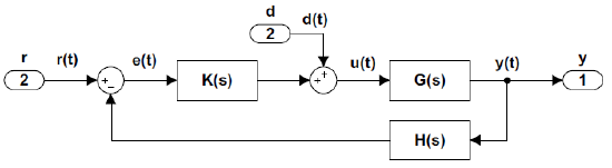
Figure \(\PageIndex{1}\): A feedback control system with reference and disturbance inputs.

Let \(r(t)\) denote a reference, and \(d(t)\) a disturbance input; then the system output is expressed in the Laplace domain as:

\[y(s)=\frac{KG(s)}{1+KGH(s)} r(s)+\frac{G(s)}{1+KGH(s)} d(s) \nonumber \]

Assuming unity-gain feedback configuration \((H(s)=1)\), the tracking error, \(e\left(s\right),\) is computed as:

\[e(s)=\frac{1}{1+KG(s)} r(s)-\frac{G(s)}{1+KG(s)} d(s) \nonumber \]

By using the FVT, the steady-state error is expressed as:

\[e(\infty )=\frac{1}{1+K_{p} } r(\infty )-\frac{G(0)}{1+K_{p} } d(\infty ) \nonumber \]

where \(K_p\) is the position error constant.

A large loop gain (large \(K_p\)) reduces steady-state error in the presence of both reference and disturbance inputs. A large controller gain, \(K\), can be used to increase \(K_p\), however, a large \(K\) would generate a large magnitude input signal to the plant, which may cause saturation in the actuator devices (amplifiers, mechanical actuators, etc.).

Simultaneous Tracking and Disturbance Rejection

To analyze the control requirements for simultaneous tracking and disturbance rejection, we consider a unity-gain feedback control system (\(H(s)=1\)).

Let \(G\left(s\right)=\frac{n\left(s\right)}{d\left(s\right)}\) represent the plant and \(K\left(s\right)=\frac{n_C\left(s\right)}{d_C\left(s\right)}\) represent the controller; then, the output in the presence of reference and disturbance inputs is given as:

\[y\left(s\right)=\frac{d\left(s\right)d_c\left(s\right)}{n\left(s\right)n_c\left(s\right)+d\left(s\right)d_c\left(s\right)}r\left(s\right)-\frac{n\left(s\right)d_c\left(s\right)}{n\left(s\right)n_c\left(s\right)+d\left(s\right)d_c\left(s\right)}d\left(s\right) \nonumber \]

The characteristic polynomial is given as: \(\Delta(s)=n(s)n_c(s)+d(s)d_c(s)\).

The requirements for asymptotic tracking and disturbance rejection are stated as follows:

Asymptotic tracking. For asymptotic tracking, \(d\left(s\right)d_c\left(s\right)\) should contain any unstable poles of \(r\left(s\right)\). For example, an integrator in the feedback loop ensures zero steady-state error to a constant reference input.

Disturbance Rejection. For disturbance rejection, \(n\left(s\right)d_c\left(s\right)\) should contain any unstable poles of \(d\left(s\right)\). For example, a notch filter centered at \(60\ Hz\) removes power line noise from the measured signal.

Example \(\PageIndex{1}\)

A small DC motor has the following component values: \(R=1\; \Omega ,\; L=10\; \rm mH,\; J=0.01\; {\rm k}g\rm m^{2} ,\; b=0.1\; \frac{\rm Ns}{\rm rad} ,k_{t} =k_{b} =0.05.\)

The DC motor transfer function is given as: \(G(s)=\frac{500}{s^{2} +110s+1025} \nonumber\).

Since \(G\left(0\right)\cong 0.5,\) with a static controller, the position error constant is: \(K_p=0.5K\). The steady-state error in the presence of reference and disturbance inputs is given as:

\[e(\infty )=\frac{1}{1+0.5K} r(\infty )-\frac{0.5}{1+0.5K} d(\infty ). \nonumber \]

We may choose a large \(K\) to reduce the steady-state tracking error as well as improve the disturbance rejection. A large value of K, however, reduces system damping and results in an oscillatory response of the DC motor.

For a static controller, the closed-loop characteristic polynomial is given as: \(\Delta (s,K)=s^{2} +110s+1025+500K.\) The resulting damping ratio is: \(\zeta =\frac{55}{\sqrt{1025+500K} }\).

In order to limit the damping to, say \(\zeta \le 0.6\), the controller gain is limited to: \(K\le 14.75\). We may choose, for example, \(K=14\), which results in the following steady-state error to reference and disturbance inputs: \(e(\infty )=\frac{1}{8} r(\infty )-\frac{1}{16} d(\infty ).\)