5.2: Static Controller Design

Static Controller Design

The RL plot displays achievable root locations for the closed-loop characteristic polynomial, \(\Delta (s)=1+KGH(s)\), as the controller gain \(K\) varies from \(0\to \infty\).

Assuming \(G(s)=\frac{n(s)}{d(s)}\), the root locus plot displays root locations for the polynomial given as: \(\Delta (s)=d(s)+Kn(s)\).

The static controller design involves the selection of the controller gain, \(K\), that marks a desired closed-loop root location on the RL plot of the loop transfer function, \(KGH(s)\).

Assuming that a RL branch passes through a desired closed-loop root location, \(s_{1}\), the associated controller gain \(K\) can be obtained from the magnitude condition, or from the MATLAB generated RL plot by clicking on that location.

Example \(\PageIndex{1}\)

Let \(KGH(s)=\frac{K}{s(s+1)(s+2)} \nonumber\); then, the closed-loop characteristic polynomial is formulated as:

\[\Delta (s)=s^{3} +3s^{2} +2s+K. \nonumber \]

Assume that we desire the closed-loop system step response to have: \(\zeta =0.7\).

From the RL plot (Figure 5.2.1), we may choose, e.g., \(K=0.66\) to satisfy this requirement. For \(K=0.66,\) the closed-loop transfer function is given as:

\[T\left(s\right)=\frac{0.66}{\left(s+2.24\right)\left(s^2+0.76s+0.29\right)} \nonumber \]

The characteristic polynomial, \(\mathit{\Delta}\left(s\right)=\left(s+2.24\right)\left(s^2+0.76s+0.29\right)\), has dominant closed-loop roots at: \(-0.38\pm 0.38\; (\zeta =0.7)\).

The step response of the closed-loop system (Figure 5.2.2) shows a 5% overshoot and a settling time of 11.5 sec.

Figure \(\PageIndex{1}\): Controller gain selection on RL plot.

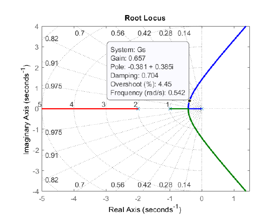
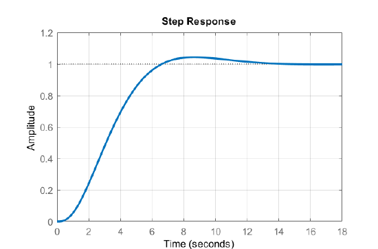
Figure \(\PageIndex{2}\): Step response of the closed-loop system.

pkg load control
s=tf('s');
Gs=1/s/(s+1)/(s+2);
rlocus(Gs)
Ts=feedback(0.657*Gs,1);
figure, step(Ts)

                                                                               
                                 Root Locus of Gs                              
                                                                               
       |-------------------------------------------------------------------|   
       |    +            +            +            +----------------**&&&-+|   
     2 |-+*****************************************|###?###asymptote&&&  +||   
       |    *            *            *            |%%%?%%%locus* &&&     ||   
       |    *            *            *            +---B---open loop poles+|   
     1 |-+****************************************************&&&********+-|   
       |    *            *            *            *   ***  &&& *          |   
       |    *            *            *            * **    &&   *          |   
     0 |##%%%%%%%%%%%%%%%%%%%%%%%%%%%%B############B@@@@@@@&&&&&B********+-|   
       |    *            *            *            *   $$$ @    *          |   
       |    *            *            *            *      $@@   *          |   
       |    *            *            *            *        @@@ *          |   
    -1 |-+****************************************************@@@********+-|   
       |    *            *            *            *            @@@        |   
       |    *            *            *            *            * @@@$     |   
    -2 |-+**********************************************************@@@$*+-|   
       |    +            +            +            +            +     @@@  |   
       |-------------------------------------------------------------------|   
           -4           -3           -2           -1            0              
                          Real Axis     gain = [0, 28.5]                       
                                                                               

 

Stability Determination from Root Locus Plot 

The range of \(K\) for closed-loop stability can be obtained from any RL branch intersection with the stability boundary, i.e., the \(j\omega\)-axis. The RL branches are likely to cross the stability boundary for \(n-m>2\).

In particular, for \(n-m=3\), the RL asymptotes are along: \({\theta }_a=\pm 60{}^\circ ,\ 180{}^\circ\). Hence, for high enough controller gains, the RL branches will cross the stability boundary leading to instability. The corresponding value of controller gain can be obtained by clicking on the RL plot.

Example \(\PageIndex{2}\)

Let \(KGH(s)=\frac{K}{s(s+1)(s+2)} \nonumber\); then, the closed-loop characteristic polynomial is:

\[\Delta (s)=s^{3} +3s^{2} +2s+K. \nonumber \]

The stability conditions for the third-order polynomial are: \(K>0,\, \, 6-K=0\). Thus, the range of \(K\) for stability is: \(0<K<6\).

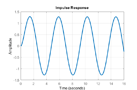
Indeed for \(K=6,\) the closed-loop characteristic polynomial, \(\mathit{\Delta}\left(s\right)=s^3+3s^2+2s+6\), has roots at: \(s=-3,\; \; \pm j\sqrt{2}\).

For \(K=6,\) the closed-loop transfer function is given as:

\[T\left(s\right)=\frac{6}{(s+3)(s^2+2)} \nonumber \]

The closed-loop system impulse response shows oscillates at the natural frequency of\(\sqrt{2}\) rad/sec (Figure 5.2.3):

Figure \(\PageIndex{3}\): Impulse response for imaginary closed-loop roots (\(K=6\)).

pkg load control
s=tf('s');
Gs=1/s/(s+1)/(s+2);
Ts=feedback(6*Gs,1);
impulse(Ts)

The static controller possesses only limited ability to a shape the response of the closed-loop system. In particular, the choice of closed-loop roots is restricted to those locations on the available root locus plot.

In the event that the existing root locus does not offer favorable pole locations, we may explore the possibility of adding a dynamic controller to the feedback loop that would modify the existing RL and cause it to pass through a desired location in the complex plane.