5.3: Transient Response Improvement

Root Locus Improvements

A dynamic controller alters the root locus plot by adding poles and zeros to the loop transfer function. In general, addition of a finite zero to the loop transfer function causes the RL branches to bend towards it, whereas, the presence of a closed-loop pole repels the RL branch close to it.

In particular, we explore the effect of adding a first-order dynamic controller, defined by: \(K(s)=\frac{K(s+z_{c} )}{s+p_{c} }\) to the feedback loop. A first-order controller adds a zero, \(-z_c\), and a pole, \(-p_c\), to the loop transfer function.

Addition of a first-order phase-lead controller to the feedback loop improves the transient response of the system; addition of a phase-lag or PI controller improves the steady-state tracking response. 

Phase-Lead Controller Design

To bring about transient response improvements, a phase-lead or a PD controller may be added to the feedback loop. A phase-lead controller is described by:

\[K\left(s\right)=\frac{K\left(s+z_c\right)}{s+p_c};\ z_c<p_c \nonumber \]

In the limiting case of \(p_c\to \infty\), the phase-lead controller changes into a PD controller, described by: \[K\left(s\right)=K\left(s+z_c\right) \nonumber \]

The PD controller has unlimited gain at high frequencies, which would amplify high-frequency noise entering the system. Thus, for effective noise suppression, a phase-lead design with \(p_c\gg z_c\) is preferred to a PD controller.

The locations of the controller pole and zero in the case of phase-lead and PD controllers are selected with the help of RL angle condition. The general design procedure is given as follow:

1. Select a desired closed-loop pole location, \(s_1\) from design specifications.
2. Compute \(G\left(s_1\right)\); the MATLAB ‘evalfr’ command can be used for this purpose.
3. Use the angle condition to determine the angle contribution required of the controller: \[{\theta }_z-{\theta }_p=180{}^\circ -\angle G\left(s_1\right) \nonumber \]
4. Select controller pole and zero locations to meet the angle contribution from the controller; since the angle condition defines a single constraint among two variables, multiple designs are possible.
5. Use the MATLAB ‘evalfr’ command to verify controller angle contribution. Note that we may only need a 'ballpark' design.
6. Plot the root locus for the compensated system and choose gain \(K\) to complete controller design.

Example \(\PageIndex{1}\): Phase-Lead Design

Let \(G(s)=\frac{2}{s(s+2)}\); design a phase-lead controller to achieve the following specifications: \(\zeta \cong 0.7,\; \; t_ s \le 2\, s\).

The phase-lead controller design proceeds as follows:

1. Let \(s_1=-2.5\pm j2.5\) describe a desired closed-loop root location.
2. By using the MATLAB ‘efalfr’ command to evaluate the plant transfer function, we get: \(G(s_1)=0.222\angle 123.7{}^\circ\); hence, the required controller phase contribution to realize the desired pole location is: \(K\left(s_1\right)=K\angle 56.3{}^\circ\). 
3. Let  \(z_c=2,\ p_c=5\); then,  \(K\left(s_1\right)=0.72\angle 55{}^\circ\).
4. Further,  \(K(s_1)G(s_1)\cong 0.16\angle 180^\circ\); hence, \(K=\frac{1}{0.16}\cong 6.3\). Alternatively, from the root locus plot of the compensated system, the controller gain is found as: \(K=6.29\); hence, \(K\left(s\right)=6.29\left(\frac{s+2}{s+5}\right)\). 

The root locus plot for the phase-lead design is shown below (Fig. 5.3.1).

Figure \(\PageIndex{1}\): Root locus for the phase-lead design.

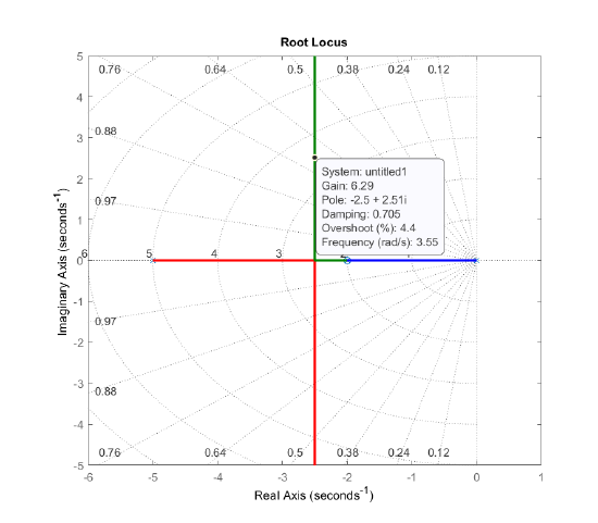
The closed-loop system is formed as: \[T(s)=\frac{12.58(s+2)}{(s+2)(s^2+5s+12.58)} \nonumber \]

We note that the closed-loop transfer function \(T(s)\) includes a pole-zero cancelation at \(s=-2\). Such cancelations are permitted as long as they are restricted to the open left-half plane (OLHP). Moreover, component inaccuracies make exact pole–zero cancelation an unlikely event in practice.

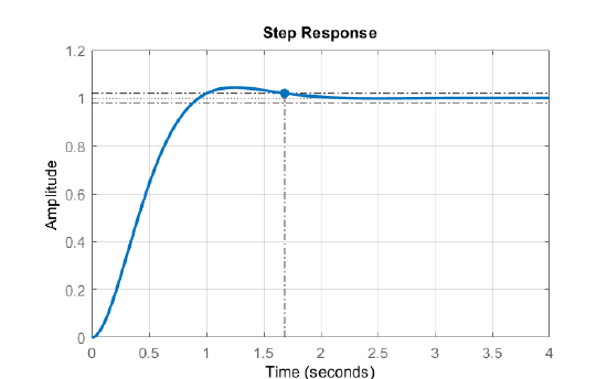
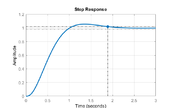
The step response of the closed-loop system is plotted in Fig. 5.3.2. From the figure, the settling time is given as: \(t_s=1.7s\).

Figure \(\PageIndex{2}\): Step response of closed-loop system.

We also note that alternate phase-lead designs for this example are possible, however, choosing controller zero location \(z_c<2\) is likely to increase the settling time of the closed-loop system.

Example \(\PageIndex{2}\): PD Controller Design

Let \(G(s)=\frac{2}{s(s+2)}\); design a PD controller to achieve the following specifications are: \(\zeta \cong 0.7,\; \; t_ s \le 2\, s\).

The PD controller design proceeds as follows:

1. Let \(s_1=-2.5\pm j2.5\) describe a desired closed-loop root location.
2. By using the MATLAB ‘efalfr’ command to evaluate the plant transfer function, we get: \(G\left(s_1\right)=0.222\angle 123.7{}^\circ\); hence, the required controller phase contribution to realize the desired pole location is: \(K\left(s_1\right)=K\angle 56.3{}^\circ\). 
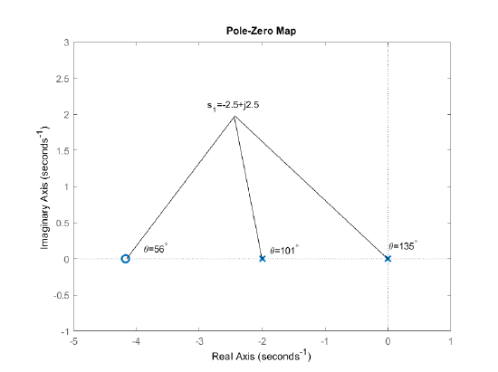
3. From trigonometry (Fig. 5.3.3), let  \(z_c=4.17\); then, for \(K(s)=s+z_c\), we have:  \(K(s_1)\cong 3\angle 56.3{}^\circ\).
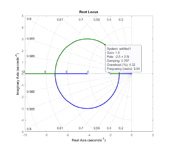
4. Since \(K(s_1)G(s_1)\cong 0.66\angle 180^\circ\), we have \(K=\frac{1}{0.66}=1.5\). Alternatively, from the RL plot of the compensated system (Fig. 5.3.4), we obtain: \(K=1.5\); hence, \(K\left(s\right)=1.5(s+4.17)\).  

Figure \(\PageIndex{3}\): Trigonometry to compute the required angle from controller zero.

Figure \(\PageIndex{4}\): Root locus plot for the PD controller.

For noise suppression considerations, it is preferable to replace the PD controller by a phase-lead design.

Accordingly, let \(K(s)=K\frac{s+4}{s+55}\); since \(K(s_1)G(s_1)\cong 0.012\angle 180^\circ\), let \(K=81.25\). Then, for \(K(s)=81.25\frac{s+4}{s+55}\), we have \(K(s_1)G(s_1)=-1\).

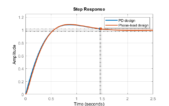
The step response of the PD controller and proposed phase-lead design are almost identical (Fig. 5.3.5).

Figure \(\PageIndex{5}\): Step response of the closed-loop systems.

A second-example of phase-lead design is presented below.

Example \(\PageIndex{3}\): Phase-Lead Design

Let \(G\left(s\right)=\frac{10}{s\left(s+2\right)(s+5)}\); assume that the design specifications are given as: \(OS\le 10\%,\ \ t_s\le 2sec\).

The phase-lead controller design proceeds as follows:

1. Let \(s_1=-2.2\pm j2.4\) describe a desired closed-loop root location.
2. Using MATLAB ‘efalfr’ command, we get: \(G\left(s_1\right)=0.35\angle 92{}^\circ\); the required controller phase contribution is: \(K\left(s_1\right)=K\angle 88{}^\circ\).
3. Let \(z_c=2,\ p_c=22\); then \(K\left(s_1\right)=0.11\angle 88{}^\circ\).
4. From the gain consideration, let \(|K(s_1)G(s_1)|=1\); then, by using 'evalfr' command, we obtain \(K=24\), hence the desired phase-lead controller is: \(K(s)=\frac{24(s+2)}{s+22}\). The compensated system has, \(K(s_1)G(s_1)\cong -1\).

The resulting closed-loop system after pole-zero cancelation is given as: \(T\left(s\right)=\frac{240}{\left(s+22.6\right)\left(s^2+4.4s+10.62\right)}\).

The step response of the closed-loop system shows a settling time of \(1.8s\).

Figure \(\PageIndex{6}\): Step response of the closed-loop system.

 

Rate Feedback Controller Design

The rate feedback configuration, shown in Figure 5.3.7, involves an inner loop with rate feedback in addition to regular output feedback. In this configuration, the rate feedback gain is \(k_f\), while \(K(s)\) denotes the outer loop controller.

Figure \(\PageIndex{7}\): Rate feedback configuration (top); equivalent diagram (bottom).

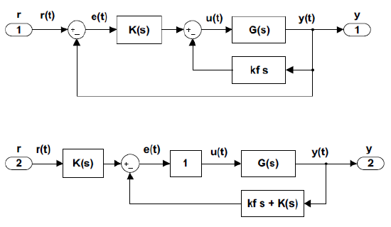
The rate feedback design is typically performed in two stages. First, the inner loop is designed for suitable closed-loop root locations. The resulting inner loop transfer function serves as a plant for the outer loop controller design.

Minor Loop Design. The loop transfer function for the minor loop is given as: \(G(s)k_ f s\). Let \(G(s)=\frac{n(s)}{d(s)}\); then, the closed-minor-loop transfer function is: \(G_{ml} (s)=\frac{n(s)}{d(s)+n(s)k_ f s} .\)

Outer Loop Design. The loop transfer function for the outer loop is given as: \(K(s)G_{ml} (s)\).

Let \(K\left(s\right)=K\); then, the closed-outer-loop transfer function is obtained as: \(T\left(s\right)=\frac{Kn\left(s\right)}{d\left(s\right)+\left(k_fs+K\right)n\left(s\right)}\).

Example \(\PageIndex{4}\)

Let \(G(s)=\frac{2}{s(s+2)}\); assume that the design specifications are given as: \(OS\le 10\%, \; t_s\le 2s \;(\zeta\ge 0.6)\).

Minor Loop Design. The minor loop gain is: \(\frac{2k_f s}{s(s+2)}\); the closed-minor-loop transfer function is: \(G_{ml} (s)=\frac{2k_f}{s(s+2+2k_f)}\).

We may select, e.g., \(k_f=1\) to obtain: \(G_{ml} (s)=\frac{2}{s(s+4)}\).

Alternatively, from the minor loop root locus (Figure 5.3.8), we select \(k_f=1\) for closed-loop root at \(s=-4\). 

Figure \(\PageIndex{8}\): Minor loop root locus.

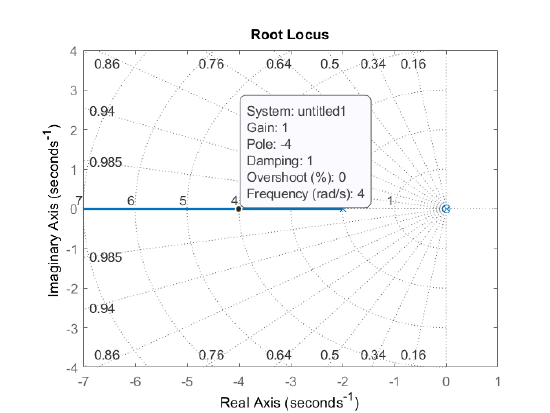
The minor loop root locus shows an apparent pole-zero cancelation at the origin. The pole at the origin is, however, retained in the outer loop design.

Outer Loop Design. The outer loop transfer function is given as: \(KG_{ml} (s)=\frac{2K}{s(s+4)}\).

From the closed-loop characteristic polynomial, \(\Delta (s)=s(s+4)+K\), we may choose, e.g., \(K=4\), for closed-loop roots to be located at: \(s=-2\pm j2\).

Alternatively, we may choose \(K=4\) from the outer loop root locus plot (Fig. 5.3.9).

Figure \(\PageIndex{9}\): Outer loop root locus.

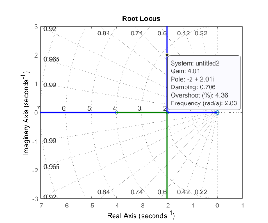
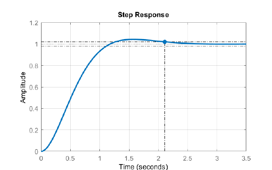
The closed-outer-loop transfer function is given as: \(T(s)=\frac{8}{s^2+4s+8}\).

The step response of the closed-loop system shows a settling time of \(2.1s\).

Figure \(\PageIndex{10}\): Step response of the closed-loop system.

Example \(\PageIndex{5}\)

Let \(G(s)=\frac{10}{s(s+2)(s+5)}\); assume that the step response specifications are: \(OS\le 10\%,\ t_s\le 2sec \; (\zeta\ge 0.6)\).

Minor Loop Design. The minor loop gain is \(k_f s\; G(s)=\frac{10k_f s}{s(s+2)(s+5)}\). From the minor loop root locus (Figure 5.3.11), we may choose, e.g., \(k_f =2\) for the closed-minor-loop roots to be located at: \(s=-3.5\pm j4.2\; (\zeta \cong 0.64)\).

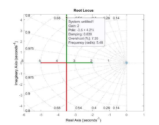
Figure \(\PageIndex{11}\): Minor loop root locus.

Outer Loop Design. The outer loop gain is obtained as: \(KG_{ml} (s)=\frac{10K}{s\left[(s+2)(s+5)+k_f \right]} =\frac{10K}{s(s^{2} +7s+30)} \).

From the outer loop root locus, we may choose, e.g., \(K=5.4\) for closed-loop roots located at: \(s=-2\pm j3.75\; (\zeta \cong 0.47)\). Although \(\zeta\) appears to be low, the step response of the closed-loop system has a small overshoot due to the presence of a real pole at \(s=-3\).

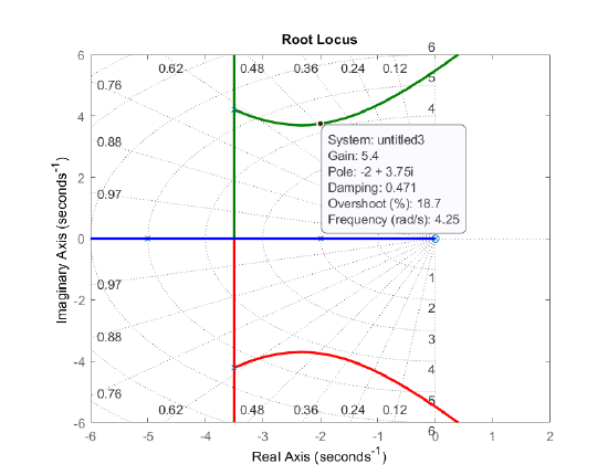
Figure \(\PageIndex{12}\): Outer loop root locus.

The closed-outer-loop transfer function is given as:  \(T(s)=\frac{54}{(s+3)(s^2+4s+18)}\).

The step response of the closed-loop system shows a settling time of \(1.5s\).

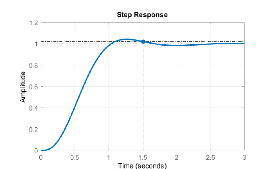
Figure \(\PageIndex{13}\): Step response of the closed-loop system.