5.4: Steady-State Error Improvement
- Page ID
- 28538

Steady-State Error Improvement
The steady-state tracking error to a step or ramp input is evaluated using the position and velocity error constants of the system. These constants are defined as:
\[K_ p ={\mathop{\lim }\limits_{s\to 0}}\; KGH(s) \nonumber \]
\[K_{v} ={\mathop{\lim }\limits_{s\to 0}}\; sKGH(s) \nonumber \]
In the case of unity-gain feedback configuration (\(H(s)=1\)), the steady-state tracking error to step and ramp inputs is computed as:
\[\left. e(\infty )\right|_{\rm step} =\frac{1}{1+K_ p } \nonumber \]
\[\left. e(\infty )\right|_{\rm ramp} =\frac{1}{K_v } \nonumber \]
where the MATLAB 'dcgain' command can be used to compute the relevant error constant.
The addition of a first-order PI or phase-lag controller to the feedback loop improves the relevant error constant. Both controllers add a pole–zero pair to the loop transfer function, and are described by:
\[K(s)=\frac{K(s+z_ c )}{(s+p_ c )} ,\quad p_ c <z_ c \nonumber \]
where \(p_c =0\) denotes the PI controller.
Assuming \(K=1\), the position error constant is raised as: \(K_p^{'} =(z_c /p_c )K_p >K_p\).
The PI controller, in particular, results in: \(K_ p^{'} =\infty\), hence \(\left. e(\infty )\right|_{\rm step} =0\). By virtue of adding an integrator to the feedback loop, the steady state error to a step input is zero for the PI controller.
Phase-Lag and PI Design
The PI/phase-lag controller design aims to boost the relevant error constant while not appreciably disturbing the existing RL plot.
Let \(s_1\) denote a desired closed-loop pole location on the existing RL plot; then, the controller pole and zero are selected in accordance with: \(p_c<z_c\ll Re(s_1)\). This ensures that the adverse angle contribution from the controller stays small, i.e., \(\theta _ z -\theta _ p \approx 0^{\circ }\).
The actual pole-zero locations for phase-lag and zero location for PI can be arbitrarily selected.
The PI/phase-lag controller adds a pole-zero pair close to the origin to the loop transfer function. Hence a closed-loop pole with a large time constant appears in the closed-loop transfer function. Nevertheless, the contribution of the added slow mode to the overall system response remains small due to the close proximity of the pole to the controller zero.
Let \(G\left(s\right)=\frac{10}{s\left(s+2\right)(s+5)}\); assume that the design specifications are given as: \(\zeta \ge 0.6,\ \ {e_{ss}|}_{\rm ramp}\le 0.1.\)
Since transient response improvement is not aimed, we may use a static controller to satisfy the damping ratio requirement.
As an example, let \(K=0.7\); then, the closed-loop system has dominant roots at: \(s=-0.8\pm j0.8\; (\zeta =0.7)\). The characteristic polynomial is factored as: \(\mathit{\Delta}\left(s\right)=(s+5.38)(s^2+1.62s+1.3)\).
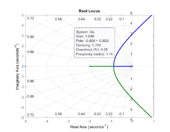
Next, the velocity error constant is evaluated as: \(K_v=0.7\).
In order to raise \(K_v>10\), we consider a phase-lag controller: \(K\left(s\right)=\frac{s+0.02}{s+0.0012}\), where \(\angle K(s_1)=-0.3{}^\circ \).
The compensated system has: \(K_v=11.67\); hence \({e_{ss}|}_{\rm ramp}\le 0.1\).
The ramp response of the closed-loop system is plotted to confirm the results.
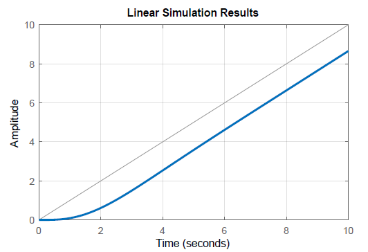
With the addition of the phase-lag controller, the closed-loop transfer function is given as:
\[T(s)=\frac{7(s+0.02)}{(s+0.0202)(s+5.38)(s^2+1.61s+1.29)} \nonumber \]
The closed-loop root at \(s=-0.0202\) is almost canceled by the presence of the zero at \(s=-0.02\). Hence, the slow mode \(e^{-0.0202t}\) has a very small coefficient and only minimally affects the system response. The dominant closed-loop roots are also minimally affected.
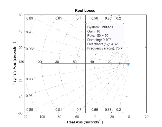
The approximate model of a DC motor is given as: \(G(s)=\frac{.5}{(.01s+1)(.1s+1)}\). The design specifications are given as: \(\zeta \ge 0.6,\ \ {e_{ss}|}_{\rm step}\le 0.01.\)
We choose a PI controller, \(K(s)=\frac{K(s+z_c)}{s}\), with unity-gain feedback \(H(s)=1\). The loop gain is given as: \(K(s)G(s)=\frac{.5K(s+z_c)}{s(.01s+1)(.1s+1)}\).
The position error constant is \(K_p=\infty\). Hence \({e_{ss}|}_{\rm step}=0\).
The controller zero can be selected to cancel one of the plant poles; hence \(z_c=10\). Next, from the RL plot, we may choose, e.g., \(K=10\). The PI controller design is given as: \(K(s)=\frac{10(s+10)}{s}\).
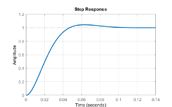
The closed-loop system transfer function is given as: \(T(s)=\frac{5000}{s^2+100s+5000}\). The step response of the closed-loop system is plotted below.