5.6: Controller Realization

Last updated
Save as PDF

Page ID: 24411

\( \newcommand{\vecs}[1]{\overset { \scriptstyle \rightharpoonup} {\mathbf{#1}} } \) \( \newcommand{\vecd}[1]{\overset{-\!-\!\rightharpoonup}{\vphantom{a}\smash {#1}}} \)\(\newcommand{\id}{\mathrm{id}}\) \( \newcommand{\Span}{\mathrm{span}}\) \( \newcommand{\kernel}{\mathrm{null}\,}\) \( \newcommand{\range}{\mathrm{range}\,}\) \( \newcommand{\RealPart}{\mathrm{Re}}\) \( \newcommand{\ImaginaryPart}{\mathrm{Im}}\) \( \newcommand{\Argument}{\mathrm{Arg}}\) \( \newcommand{\norm}[1]{\| #1 \|}\) \( \newcommand{\inner}[2]{\langle #1, #2 \rangle}\) \( \newcommand{\Span}{\mathrm{span}}\) \(\newcommand{\id}{\mathrm{id}}\) \( \newcommand{\Span}{\mathrm{span}}\) \( \newcommand{\kernel}{\mathrm{null}\,}\) \( \newcommand{\range}{\mathrm{range}\,}\) \( \newcommand{\RealPart}{\mathrm{Re}}\) \( \newcommand{\ImaginaryPart}{\mathrm{Im}}\) \( \newcommand{\Argument}{\mathrm{Arg}}\) \( \newcommand{\norm}[1]{\| #1 \|}\) \( \newcommand{\inner}[2]{\langle #1, #2 \rangle}\) \( \newcommand{\Span}{\mathrm{span}}\)\(\newcommand{\AA}{\unicode[.8,0]{x212B}}\)

Frequency Selective Filters

The dynamic controllers, including phase-lead, phase-lag, lead-lag, PD, PI, PID, represent frequency selective filters that may be realized by electronic circuits built with operational amplifiers and resistor-capacitor networks.

A resister-capacitor (RC) circuit connected in series or parallel has the following impedance:

Series RC circuit: \(Z_{\rm ser} (s)=R+\frac{1}{C\rm s} =\frac{RCs+1}{Cs}\)

Parallel RC circuit: \(Z_{\rm par} (s)=\frac{R/Cs}{R+\frac{1}{Cs} } =\frac{R}{RCs+1}\)

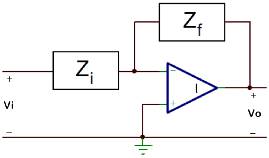
An operational amplifier (Op-Amp) in the inverting configuration has an input–output transfer function: \(\frac{V_{0} (s)}{V_\rm i (s)} =-\frac{Z_\rm f (s)}{Z_\rm i (s)} ,\) where \(Z_\rm i (s)\) and \(Z_\rm f (s)\) denote the input and feedback path impedance.

Figure \(\PageIndex{1}\): Operational amplifier in the inverting configuration

Phase-Lead/Phase-Lag Controllers

A first-order phase-lead or phase-lag controller can be realized with parallel RC circuits placed as input and feedback paths. The resulting controller transfer function is given as:

\[K(s)=-\frac{Z_\rm f (s)}{Z_\rm i (s)} =-\frac{R_{f} }{R_{i} } \frac{(R_\rm i C_\rm i s+1)}{(R_\rm f C_\rm f s+1)} . \nonumber \]

The controller transfer function has a zero located at: \(z_\rm c =\frac{1}{R_\rm i C_\rm i }\), and a pole at: \(p_\rm c =\frac{1}{R_\rm f C_\rm f }\).

Hence we may choose \(R_{\rm i} C_{\rm i} >R_{\rm f} C_{\rm f}\) for the phase-lead and \(R_{\rm i} C_{\rm i} <R_{\rm f} C_{\rm f}\) for the phase-lag design.

For static gain and sign correction, a resistive Op-Amp circuit can be employed. The circuit has a gain of: \(\frac{V_{\rm o} }{V_\rm i } =-\frac{R_{\rm f} }{R_{\rm i} } \).

Example \(\PageIndex{1}\)

Let \(K(s)=\frac{5(s+1)}{s+10}=\frac{0.5(s+1)}{0.1s+1}\); then, the transfer function realization involves the following constraints: \(R_{\rm i} C_{\rm i} =1,\; R_{\rm f} C_{\rm f} =0.1,\; R_{\rm f} /R_\rm i =0.5.\)

We may choose, for example, \(R_\rm i =100K\Omega\). Then, \(R_\rm f =50K\, \Omega ,\; C_\rm i =10\mu \, {\rm F},\; C_\rm f =2\mu \, {\rm F.}\;\)

PD, PI, PID Controllers

These controllers can be realized by combining the following impedance:

\[G_{\rm PD} (s)=-\frac{R_\rm f }{Z_{\rm par} (s)} =-\frac{R_\rm f }{R_\rm i } (R_\rm i C_\rm i s+1) \nonumber \]

\[G_{\rm PI} (s)=-\frac{1/C_\rm f s}{Z_{\rm par} (s)} =-\frac{1}{R_\rm i C_\rm f } \frac{(R_\rm i C_\rm i s+1)}{s} \nonumber \]

\[G_{\rm PID} (s)=-\frac{Z_{\rm f-ser} (s)}{Z_{\rm i-par} (s)} =-\frac{1}{R_\rm i C_\rm f } \frac{(R_\rm i C_\rm i s+1)(R_\rm f C_\rm f s+1)}{s} . \nonumber \]

For the PID controller, the controller gains are solved as functions of component values:

\[\rm k_\rm p =\frac{R_{\rm f} }{R_{\rm i} } +\frac{C_{\rm i} }{C_{\rm f} } ,\; \; k_\rm i =R_{\rm f} C_{\rm i},\; \; k_\rm d =\frac{1}{R_{\rm i} C_{\rm f} } \nonumber \]

Example \(\PageIndex{2}\)

Let \(G_{\rm PID} (s)=\frac{(s+0.1)(s+10)}{s}\); then, to realize the transfer function with RC networks, we may choose, for example:

\[R_{\rm i} =100\; {\rm K}\Omega ,\; R_{\rm f} =1{\rm M}\Omega ,\; C_{\rm i} =1\; \mu \, {\rm F},\; C_{\rm f} =10\; \mu \, {\rm F} \nonumber \]